Case Study: Bering Sea and Aleutian Islands Blackspotted and Rougheye Rockfish
Source:vignettes/z_bsai_rougheye_rockfish_case_study.Rmd
z_bsai_rougheye_rockfish_case_study.RmdOverview
This case study reproduces the 2024 Bering Sea and Aleutian Islands
blackspotted and rougheye rockfish assessment in SPoRC.
Every structural choice below follows the assessment rather than
SPoRC’s defaults.
The model is single region, single sex, single season, with one fishery fleet and one survey:
| Source | Years | Observations | Likelihood |
|---|---|---|---|
| Catch | 1977–2024 | 48 | Lognormal, weighted |
| Aleutian Islands survey biomass | 1991–2024 | 14 | Lognormal |
| Fishery age compositions | 2004–2023 | 13 | Multinomial |
| Fishery length compositions | 1979–2022 | 11 | Multinomial |
| Survey age compositions | 1991–2022 | 13 | Multinomial |
| Survey length compositions | 2024 | 1 | Multinomial |
Model ages run 3 to 54 with a plus group, while the assessment reports over observed ages 3 to 45 with its last column pooling the model’s ages 45 to 54. Lengths run 12 to 50 cm.
Model dimensions
Because the model is single region and single sex, the population, region, season and sex subscripts used in the model equations all collapse to one, and are dropped from the notation below.
input_list <- Setup_Mod_Dim(
  n_pop = dat$n_pop,
  years = yrs,
  ages = dat$ages,
  lens = dat$lens,
  n_regions = dat$n_regions,
  n_sexes = dat$n_sexes,
  n_fish_fleets = dat$n_fish_fleets,
  n_srv_fleets = dat$n_srv_fleets,
  n_seas = dat$n_seas,
  bias_correct_pe = "none", # the assessment corrects neither recruitment nor the initial ages
  verbose = FALSE
)
Recruitment and the initial age structure
Recruitment is a mean with annual deviations rather than a stock recruit function, and the last three years take the mean outright:
The initial age structure is where this assessment differs most from
a SPoRC default. Its fyear_ac_option 3 gives
the first year its own scalar, independent of the recruitment level,
with deviations that ages beyond the observed range share:
use_rinit = 1 is what creates that separate scalar, and
equil_init_age_strc = "stoch_shared_ages" with an explicit
init_age_devs_shared vector is what makes the ages past the
observed range share the last deviation. Here the observed range runs to
age 45, so the deviations are free over the first 42 ages and the final
nine share the 42nd. SPoRC holds the initial numbers as
multiplicative deviations from an equilibrium age structure rather than
as the structure itself, so the seeding step below converts between the
two.
input_list <- Setup_Mod_Rec(
  input_list = input_list,
  rec_model = "mean_rec",
  sigmaR_switch = 1,
  ln_sigmaR = array(log(dat$sigmaR), dim = c(2, dat$n_pop, dat$n_regions)),
  equil_init_age_strc = "stoch_shared_ages",
  init_age_devs_shared = c(1:42, rep(42, 9)),
  dont_est_recdev_last = 3,
  sigmaR_spec = "fix",
  init_age_strc = 1,
  t_spawn = (3 - 1) / 12,
  use_rinit = 1
)
Biological dynamics
Natural mortality is estimated under a lognormal prior. The
assessment states its prior as a mean of
on the natural scale, so the median supplied to SPoRC is
shifted by
to put the prior mean where the assessment puts it:
input_list <- Setup_Mod_Biologicals(
  input_list = input_list,
  WAA = dat$WAA,
  MatAA = dat$MatAA,
  fit_lengths = 1,
  SizeAgeTrans = dat$SizeAgeTrans,
  AgeingError = dat$AgeingError,
  M_spec = "est_ln_M",
  Use_M_prior = 1,
  M_prior = data.frame(popblk = 1, regionblk = 1, yearblk = 1, ageblk = 1, sexblk = 1,
                       mu = dat$mean_M * exp(-dat$cv_M^2 / 2), sd = dat$cv_M),
  addtosrvidx = 1e-13,
  addtocomp = 1e-13
)
Movement and tagging
The model is single region, so movement is an identity matrix and no tagging data are used. Both still have to be declared.
input_list <- Setup_Mod_Movement(input_list = input_list, use_fixed_movement = 1,
                                 Fixed_Movement = NA, do_recruits_move = 0)

input_list <- Setup_Mod_Tagging(input_list = input_list, use_conv_fish_tagging = 0)
Catch and fishing mortality
The assessment writes its catch and F statements as weighted sums of squares with weights and . A weighted sum of squares and a normal likelihood with a fixed standard deviation are the same statement up to a constant, related by , so both weights are kept inside the standard deviations rather than applied outside the sums.
suppressWarnings(
  input_list <- Setup_Mod_Catch_and_F(
    input_list = input_list,
    ObsCatch = dat$ObsCatch,
    UseCatch = dat$UseCatch,
    Use_F_pen = 1,
    sigmaC_spec = "fix",
    ln_sigmaC = array(log(sqrt(1 / (2 * 50))),
                      dim = c(dat$n_regions, n_yrs, dat$n_seas, dat$n_fish_fleets)),
    ln_sigmaF = array(log(sqrt(1 / (2 * 0.1))),
                      dim = c(dat$n_regions, dat$n_seas, dat$n_fish_fleets))
  )
)
Fishery compositions
There is no fishery index in this assessment, only compositions, so
fish_idx_type is "none" and the index arrays
are declared empty.
input_list <- Setup_Mod_FishIdx_and_Comps(
  input_list = input_list,
  ObsFishIdx = array(NA, dim = c(dat$n_regions, n_yrs, dat$n_seas, dat$n_fish_fleets)),
  ObsFishIdx_SE = array(NA, dim = c(dat$n_regions, n_yrs, dat$n_seas, dat$n_fish_fleets)),
  UseFishIdx = array(0, dim = c(dat$n_regions, n_yrs, dat$n_seas, dat$n_fish_fleets)),
  ObsFishAgeComps = dat$ObsFishAgeComps,
  UseFishAgeComps = dat$UseFishAgeComps,
  ISS_FishAgeComps = dat$ISS_FishAgeComps,
  ObsFishLenComps = dat$ObsFishLenComps,
  UseFishLenComps = dat$UseFishLenComps,
  ISS_FishLenComps = dat$ISS_FishLenComps,
  fish_idx_type = "none",
  FishAgeComps_LikeType = "Multinomial",
  FishLenComps_LikeType = "Multinomial",
  FishAgeComps_Type = "agg_Year_1-terminal_Fleet_1",
  FishLenComps_Type = "agg_Year_1-terminal_Fleet_1"
)
Survey index and compositions
The Aleutian Islands bottom trawl survey supplies a biomass index, age compositions, and a single year of length compositions. The index is lognormal with year specific standard errors, and the survey is fit at mid year.
input_list <- Setup_Mod_SrvIdx_and_Comps(
  input_list = input_list,
  ObsSrvIdx = dat$ObsSrvIdx,
  ObsSrvIdx_SE = dat$ObsSrvIdx_SE,
  UseSrvIdx = dat$UseSrvIdx,
  ObsSrvAgeComps = dat$ObsSrvAgeComps,
  ISS_SrvAgeComps = dat$ISS_SrvAgeComps,
  UseSrvAgeComps = dat$UseSrvAgeComps,
  ObsSrvLenComps = dat$ObsSrvLenComps,
  UseSrvLenComps = dat$UseSrvLenComps,
  ISS_SrvLenComps = dat$ISS_SrvLenComps,
  srv_idx_type = "biom",
  SrvAgeComps_LikeType = "Multinomial",
  SrvLenComps_LikeType = "Multinomial",
  SrvAgeComps_Type = "agg_Year_1-terminal_Fleet_1",
  SrvLenComps_Type = "agg_Year_1-terminal_Fleet_1"
)
Fishery selectivity and catchability
Both fleets use the slope and
parameterization of the logistic, which is logist1:
Selectivity is time invariant, so there are no deviations and no process error. Fishery catchability is not used, because there is no fishery index to scale.
input_list <- Setup_Mod_Fishsel_and_Q(
  input_list = input_list,
  cont_tv_fish_sel = "none_Fleet_1",
  fish_sel_blocks = "none_Fleet_1",
  fish_sel_model = "logist1_Fleet_1",
  fish_q_blocks = "none_Fleet_1",
  fish_fixed_sel_pars_spec = "est_all",
  fish_q_spec = "fix"
)
Survey selectivity and catchability
Survey selectivity takes the same logistic form. Catchability is estimated under a lognormal prior centered on with a coefficient of variation of , with the same shift applied to the median so the prior mean lands where the assessment puts it.
input_list <- Setup_Mod_Srvsel_and_Q(
  input_list = input_list,
  cont_tv_srv_sel = "none_Fleet_1",
  srv_sel_blocks = "none_Fleet_1",
  srv_sel_model = "logist1_Fleet_1",
  srv_q_blocks = "none_Fleet_1",
  srv_fixed_sel_pars_spec = "est_all",
  srv_q_spec = "est_all",
  Use_srv_q_prior = 1,
  srv_q_prior = data.frame(region = 1, block = 1, fleet = 1,
                           mu = dat$mean_q * exp(-dat$cv_q^2 / 2), sd = dat$cv_q),
  t_srv = array(0.5, dim = c(dat$n_regions, dat$n_seas, dat$n_srv_fleets))
)
Weighting
The catch and F weights are already inside their standard deviations, so the only weights left are the composition multipliers, which are the assessment’s stage 2 values and ship in the data object.
input_list <- Setup_Mod_Weighting(
  input_list = input_list,
  Wt_Catch = 1, Wt_FishIdx = 1, Wt_SrvIdx = 1,
  Wt_Rec = 1, Wt_F = 1, Wt_Tagging = 0,
  Wt_FishAgeComps = dat$Wt_FishAgeComps,
  Wt_FishLenComps = dat$Wt_FishLenComps,
  Wt_SrvAgeComps = dat$Wt_SrvAgeComps,
  Wt_SrvLenComps = dat$Wt_SrvLenComps
)
Starting at the ADMB estimate
Before optimizing anything, check that the model is reproduced at a known point. Setting every parameter to the assessment’s maximum likelihood estimate and evaluating there separates a specification error from an optimization difference: if the population and the likelihood agree at the ADMB solution, the two models are the same model.
Most parameters can be assigned directly. The recruitment deviations
are seeded only over the years the assessment estimates them for, and
the initial age structure needs the conversion described above: the
assessment writes the first year directly, while SPoRC has
multiplicative deviations from an equilibrium age structure, so the
deviations are the log ratio of the two.
mle <- dat$mle

input_list$par$ln_global_R0[] <- mle$mean_log_rec
input_list$par$ln_rinit <- mle$log_rinit
input_list$par$ln_M[] <- log(mle$M)
input_list$par$ln_srv_q[] <- log(mle$q_srv)
input_list$par$ln_F_mean[] <- mle$log_avg_fmort
input_list$par$ln_F_devs[1, , 1, 1] <- mle$fmort_dev
input_list$par$fish_fixed_sel_pars[] <- log(c(mle$sel_a50_fish, mle$sel_aslope_fish))
input_list$par$srv_fixed_sel_pars[] <- log(c(mle$sel_a50_srv, mle$sel_aslope_srv))
input_list$par$ln_RecDevs[1, 1, seq_along(mle$rec_dev)] <- mle$rec_dev

# The assessment's initial numbers at age against SPoRC's equilibrium reference.
NAA_equil <- exp(mle$log_rinit) * exp(-(0:(n_ages - 1)) * mle$M)
NAA_equil[n_ages] <- NAA_equil[n_ages - 1] * exp(-mle$M) / (1 - exp(-mle$M))
NAA_styr <- NAA_equil
for(j in 2:n_obs_ages) {
  NAA_styr[j] <- exp(mle$log_rinit - mle$M * (j - 1) + mle$fydev[j - 1])
} # end j loop
for(j in (n_obs_ages + 1):n_ages) {
  NAA_styr[j] <- exp(mle$log_rinit - mle$M * (j - 1) + mle$fydev[length(mle$fydev)])
} # end j loop
NAA_styr[n_ages] <- exp(mle$log_rinit - mle$M * (n_ages - 1) +
                          mle$fydev[length(mle$fydev)]) / (1 - exp(-mle$M))
input_list$par$ln_InitDevs[1, 1, , ] <- (log(NAA_styr) - log(NAA_equil))[-1]

obj <- fit_model(input_list$data, input_list$par, input_list$map,
                 do_optim = FALSE, silent = TRUE)
r <- obj$rep
At that point every reported quantity agrees with the ADMB model:
fishery selectivity max pct diff: 4.3e-04
survey selectivity  max pct diff: 4.2e-04
numbers at age, 4+  max pct diff: 4.9e-04
spawning biomass    max pct diff: 7.7e-03
fishing mortality   max pct diff: 3.7e-04
jnLL at the assessment MLE: 297.5081
max |gradient| there      : 0.0864
The gradient at the seed point is small but not zero, which is what an ADMB maximum likelihood estimate reported to six significant figures looks like when it is read back in.
Recruitment splits into two windows. Over the years the assessment
estimates a deviation for, the two agree outright. Over the terminal
three years the assessment multiplies mean recruitment by
while leaving the estimated recruitments uncorrected, so
SPoRC sits exactly that factor low: the observed ratio is
against
.
This is a convention difference and not an error. It moves terminal
spawning biomass by
percent, because maturity at age 3 is
.
Fitting and comparison
est <- fit_model(input_list$data, input_list$par, input_list$map,
                 random = NULL, newton_loops = 3, silent = TRUE)
est$sdrep <- RTMB::sdreport(est)
free parameters: 144
final jnLL: 297.508 max |gradient|: 9.1e-13
pdHess: TRUEThe optimized objective is the value the seed point already had, to
four decimal places, so the assessment’s maximum likelihood estimate is
SPoRC’s optimum as well.
| Quantity | Median difference | Maximum difference |
|---|---|---|
| Spawning biomass | 0.034 % | 0.051 % |
| Recruitment, estimated years | 0.043 % | 0.263 % |
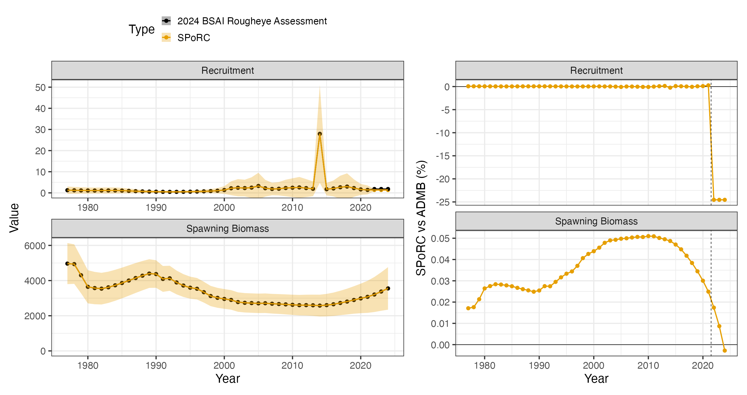
| Recruitment, terminal three | 24.5 % | 24.5 % |
The last row is the bias correction convention described above, at its exact expected size of , and it is why the dashed rule in the figure marks where the estimated deviations stop.
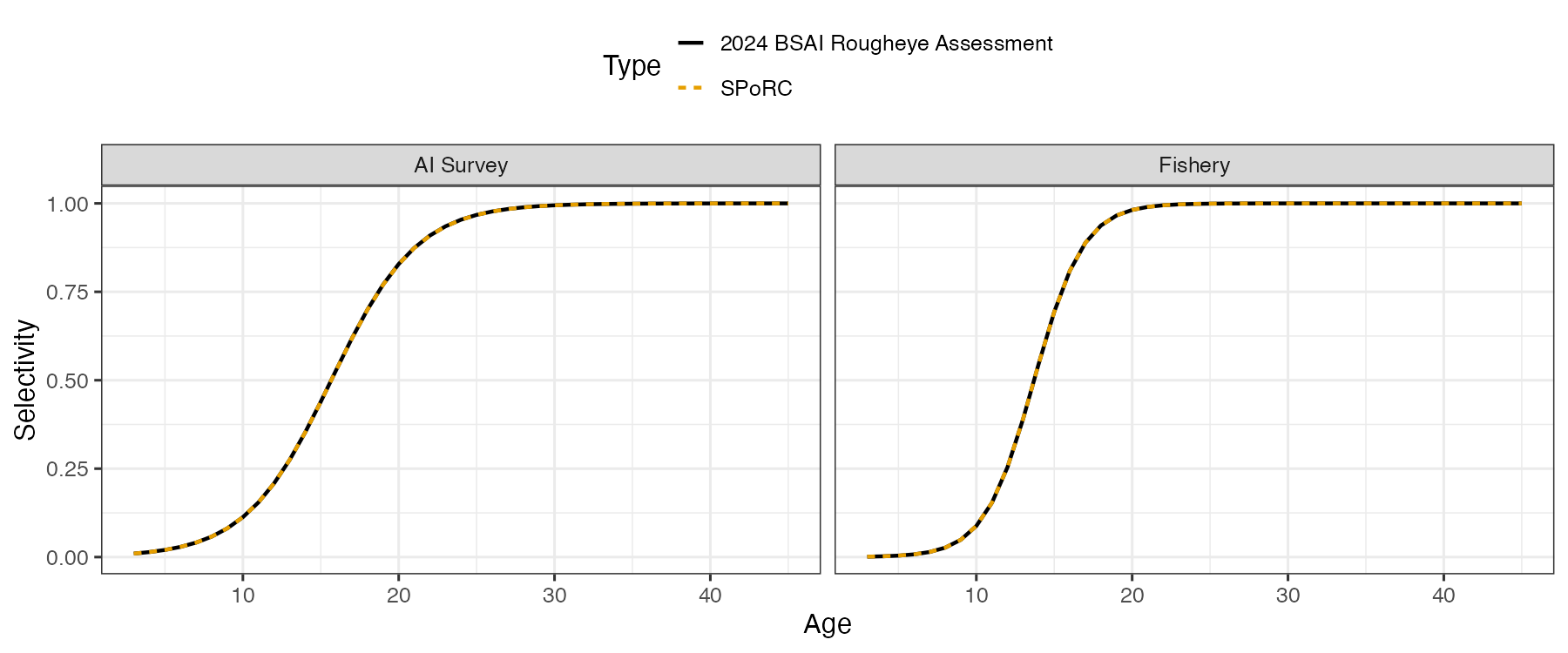
Selectivity is time invariant in both fleets, so a single curve per fleet suffices.