Case Study: Gulf of Alaska Northern Rockfish
Source:vignettes/w_goa_northern_rockfish_case_study.Rmd
w_goa_northern_rockfish_case_study.RmdOverview
This case study reproduces the 2024 Gulf of Alaska northern rockfish
assessment in SPoRC. Every structural choice below follows
the assessment rather than SPoRC’s defaults, and the result
is an exact bridge: evaluated at the assessment’s own maximum likelihood
estimate, spawning biomass agrees to
percent and every likelihood component reproduces to six significant
figures.
The model is single region, single sex, single season, with one fishery fleet and one survey:
| Source | Years | Observations | Likelihood |
|---|---|---|---|
| Catch | 1961–2024 | 64 | Lognormal, weighted |
| Bottom trawl survey biomass | 1990–2023 | 16 | Lognormal |
| Fishery age compositions | 1998–2022 | 16 | Multinomial |
| Fishery length compositions | 1991–2023 | 17 | Multinomial |
| Survey age compositions | 1990–2023 | 16 | Multinomial |
Model ages run 2 to 51 with a plus group, while the assessment reports over observed ages 2 to 45. Lengths run 15 to 45 cm.
library(SPoRC)
library(dplyr)
library(ggplot2)
data("sgl_rg_goa_nork_data")

dat <- sgl_rg_goa_nork_data
yrs <- dat$years
n_yrs <- length(yrs)
n_ages <- length(dat$ages)
The object has three kinds of content: the model inputs
(ObsCatch, WAA, ObsSrvIdx, and so
on), the ADMB maximum likelihood estimate in dat$mle, used
both as a starting point and to verify the objective before any
optimization, and the ADMB output in dat$admb, which is the
comparison target.
Model dimensions
Because the model is single region and single sex, the population, region, season and sex subscripts used in the model equations all collapse to one, and are dropped from the notation below.
input_list <- Setup_Mod_Dim(
  n_pop = dat$n_pop,
  years = yrs,
  ages = dat$ages,
  lens = dat$lens,
  n_regions = dat$n_regions,
  n_sexes = dat$n_sexes,
  n_fish_fleets = dat$n_fish_fleets,
  n_srv_fleets = dat$n_srv_fleets,
  n_seas = dat$n_seas,
  verbose = FALSE
)
Recruitment
Recruitment is a mean with annual deviations rather than a stock recruit function:
with
fixed. There is no lognormal bias correction, so
do_rec_bias_ramp = 0 and the penalty is centered on zero,
which is what the ADMB template does. Every year has a deviation,
including the terminal years, so dont_est_recdev_last = 0.
The first year sits in an unfished equilibrium age structure with its
own deviations, which is init_age_strc = 1, and spawning
occurs at the start of the year.
input_list <- Setup_Mod_Rec(
  input_list = input_list,
  rec_model = "mean_rec",
  do_rec_bias_ramp = 0,
  sigmaR_switch = 1,
  ln_sigmaR = array(log(dat$sigmaR), dim = c(2, dat$n_pop, dat$n_regions)),
  dont_est_recdev_last = 0,
  sigmaR_spec = "fix",
  init_age_strc = 1,
  t_spawn = 0
)
Biological dynamics
Natural mortality is estimated under a lognormal prior centered on with a coefficient of variation of :
Length compositions are fit through a size at age transition matrix, and age compositions pass through an ageing error matrix, so both are declared here rather than at the composition call.
input_list <- Setup_Mod_Biologicals(
  input_list = input_list,
  WAA = dat$WAA,
  MatAA = dat$MatAA,
  fit_lengths = 1,
  SizeAgeTrans = dat$SizeAgeTrans,
  AgeingError = dat$AgeingError,
  M_spec = "est_ln_M",
  Use_M_prior = 1,
  M_prior = data.frame(popblk = 1, regionblk = 1, yearblk = 1, ageblk = 1, sexblk = 1,
                       mu = dat$mean_M, sd = dat$cv_M),
  addtosrvidx = 0.00001,
  addtocomp = 0.00001
)
Movement and tagging
The model is single region, so movement is an identity matrix and no tagging data are used. Both still have to be declared.
input_list <- Setup_Mod_Movement(input_list = input_list, use_fixed_movement = 1,
                                 Fixed_Movement = NA, do_recruits_move = 0)

input_list <- Setup_Mod_Tagging(input_list = input_list, use_conv_fish_tagging = 0)
Catch and fishing mortality
The assessment writes its catch and F statements as weighted sums of
squares. A weighted sum of squares and a normal likelihood with a fixed
standard deviation are the same statement up to a constant, related by
,
so the weights enter through ln_sigmaC and
ln_sigmaF rather than through a separate multiplier:
The reconstructed catches before 1978 have a weight of and the observer era series a weight of , which is the assessment’s way of saying the early series is less certain. The F deviations have with the overall weight of applied in the weighting section.
ln_sigmaC <- array(NA_real_, dim = c(dat$n_regions, n_yrs, dat$n_seas, dat$n_fish_fleets))
ln_sigmaC[1, , 1, 1] <- log(sqrt(1 / (2 * dat$catch_wt)))

suppressWarnings(
  input_list <- Setup_Mod_Catch_and_F(
    input_list = input_list,
    ObsCatch = dat$ObsCatch,
    UseCatch = dat$UseCatch,
    Use_F_pen = 1,
    sigmaC_spec = "fix",
    ln_sigmaC = ln_sigmaC,
    ln_sigmaF = array(log(sqrt(1 / 2)),
                      dim = c(dat$n_regions, dat$n_seas, dat$n_fish_fleets))
  )
)
Fishery compositions
There is no fishery index in this assessment, only compositions, so
fish_idx_type is "none" and the index arrays
are declared empty. Both age and length compositions are aggregated over
the region and fit multinomially.
input_list <- Setup_Mod_FishIdx_and_Comps(
  input_list = input_list,
  ObsFishIdx = array(NA, dim = c(dat$n_regions, n_yrs, dat$n_seas, dat$n_fish_fleets)),
  ObsFishIdx_SE = array(NA, dim = c(dat$n_regions, n_yrs, dat$n_seas, dat$n_fish_fleets)),
  UseFishIdx = array(0, dim = c(dat$n_regions, n_yrs, dat$n_seas, dat$n_fish_fleets)),
  ObsFishAgeComps = dat$ObsFishAgeComps,
  UseFishAgeComps = dat$UseFishAgeComps,
  ISS_FishAgeComps = dat$ISS_FishAgeComps,
  ObsFishLenComps = dat$ObsFishLenComps,
  UseFishLenComps = dat$UseFishLenComps,
  ISS_FishLenComps = dat$ISS_FishLenComps,
  fish_idx_type = "none",
  FishAgeComps_LikeType = "Multinomial",
  FishLenComps_LikeType = "Multinomial",
  FishAgeComps_Type = "agg_Year_1-terminal_Fleet_1",
  FishLenComps_Type = "agg_Year_1-terminal_Fleet_1"
)
Survey index and compositions
The bottom trawl survey supplies a biomass index and age
compositions. The index is lognormal with year specific standard errors,
and the survey is fit at the start of the year, which
t_srv = 0 sets in the selectivity section below.
input_list <- Setup_Mod_SrvIdx_and_Comps(
  input_list = input_list,
  ObsSrvIdx = dat$ObsSrvIdx,
  ObsSrvIdx_SE = dat$ObsSrvIdx_SE,
  UseSrvIdx = dat$UseSrvIdx,
  ObsSrvAgeComps = dat$ObsSrvAgeComps,
  ISS_SrvAgeComps = dat$ISS_SrvAgeComps,
  UseSrvAgeComps = dat$UseSrvAgeComps,
  ObsSrvLenComps = dat$ObsSrvLenComps,
  UseSrvLenComps = dat$UseSrvLenComps,
  ISS_SrvLenComps = dat$ISS_SrvLenComps,
  srv_idx_type = "biom",
  SrvAgeComps_LikeType = "Multinomial",
  SrvLenComps_LikeType = "Multinomial",
  SrvAgeComps_Type = "agg_Year_1-terminal_Fleet_1",
  SrvLenComps_Type = "agg_Year_1-terminal_Fleet_1"
)
Fishery selectivity and catchability
Both fleets use the
and
parameterization of the logistic, which is logist2:
Selectivity is time invariant, so there are no deviations and no process error. Fishery catchability is not used, because there is no fishery index to scale.
input_list <- Setup_Mod_Fishsel_and_Q(
  input_list = input_list,
  cont_tv_fish_sel = "none_Fleet_1",
  fish_sel_blocks = "none_Fleet_1",
  fish_sel_model = "logist2_Fleet_1",
  fish_q_blocks = "none_Fleet_1",
  fish_fixed_sel_pars_spec = "est_all",
  fish_q_spec = "fix"
)
Survey selectivity and catchability
Survey selectivity takes the same logistic form. Catchability is estimated under a lognormal prior centered on with a coefficient of variation of , which is loose enough to let the data move it:
input_list <- Setup_Mod_Srvsel_and_Q(
  input_list = input_list,
  cont_tv_srv_sel = "none_Fleet_1",
  srv_sel_blocks = "none_Fleet_1",
  srv_sel_model = "logist2_Fleet_1",
  srv_q_blocks = "none_Fleet_1",
  srv_fixed_sel_pars_spec = "est_all",
  srv_q_spec = "est_all",
  Use_srv_q_prior = 1,
  srv_q_prior = data.frame(region = 1, block = 1, fleet = 1,
                           mu = dat$mean_q, sd = dat$cv_q),
  t_srv = array(0, dim = c(dat$n_regions, dat$n_seas, dat$n_srv_fleets))
)
Weighting
The survey index has a weight of and the F penalty a weight of . Every composition source holds the assessment’s own multipliers, which ship in the data object.
input_list <- Setup_Mod_Weighting(
  input_list = input_list,
  Wt_Catch = 1, Wt_FishIdx = 1, Wt_SrvIdx = dat$srv_wt,
  Wt_Rec = 1, Wt_F = dat$fmort_wt, Wt_Tagging = 0,
  Wt_FishAgeComps = dat$Wt_FishAgeComps,
  Wt_FishLenComps = dat$Wt_FishLenComps,
  Wt_SrvAgeComps = dat$Wt_SrvAgeComps,
  Wt_SrvLenComps = dat$Wt_SrvLenComps
)
Starting at the ADMB estimate
Before optimizing anything, check that the model is reproduced at a known point. Setting every parameter to the assessment’s maximum likelihood estimate and evaluating there separates a specification error from an optimization difference: if the population and the likelihood agree at the ADMB solution, the two models are the same model.
Every parameter can be assigned directly here, because recruitment is a mean with deviations rather than a stock recruit function and nothing has to be solved by substitution. The initial age deviations were back derived from the ADMB numbers at age when the data object was built, so seeding them reproduces the ADMB starting conditions exactly.
mle <- dat$mle

input_list$par$ln_global_R0[] <- mle$log_mean_R
input_list$par$ln_RecDevs[1, 1, ] <- mle$log_Rt
input_list$par$ln_InitDevs[1, 1, , ] <- mle$init_devs
input_list$par$ln_M[] <- log(mle$M)
input_list$par$ln_F_mean[] <- mle$log_mean_F
input_list$par$ln_F_devs[1, , 1, 1] <- mle$log_Ft
input_list$par$fish_fixed_sel_pars[] <- log(c(mle$a50C, mle$deltaC))
input_list$par$srv_fixed_sel_pars[] <- log(c(mle$a50S, mle$deltaS))
input_list$par$ln_srv_q[] <- log(mle$q)

obj <- fit_model(input_list$data, input_list$par, input_list$map,
                 do_optim = FALSE, silent = TRUE)
r <- obj$rep
At that point every reported quantity agrees with the ADMB model to numerical precision:
fishery selectivity max pct diff: 5.5e-08
survey selectivity  max pct diff: 2.7e-08
numbers at age      max pct diff: 1.5e-08
spawning biomass    max pct diff: 7.5e-09
recruitment         max pct diff: 4.7e-14
The likelihood is checked the same way. SPoRC writes
each component as a proper density while the assessment drops
normalizing constants, so a like for like comparison subtracts exactly
the constants the assessment omits. The catch statement is a weighted
sum of squares, so subtracting SPoRC’s per observation
leaves it. The survey statement keeps its
term but drops
.
The recruitment penalty is the sum of squares over the recruitment
deviations and the initial age deviations together, with no constants at
all.
| Component | SPoRC |
Assessment |
|---|---|---|
| Catch sum of squares | 0.0994676 | 0.0994676 |
| Survey index | -0.6442737 | -0.6442737 |
| Fishery age compositions | 46.3671 | 46.3700 |
| Fishery length compositions | 63.1396164 | 63.1396164 |
| Survey age compositions | 84.3318 | 84.3389 |
| Recruitment | 9.9131179 | 9.9131179 |
| F regularity | 5.7786429 | 5.7786429 |
| prior | 0.0406345 | 0.0406345 |
| prior | 0.1734080 | 0.1734080 |
Seven of the nine components are exact. The two age composition terms agree to about relative, which is the two templates’ different robustifying constants inside the multinomial and not a difference in the compositions themselves.
Fitting and comparison
Optimizing from that point moves very little, which is the expected result when a model is already close to its own optimum.
est <- fit_model(input_list$data, input_list$par, input_list$map,
                 random = NULL, newton_loops = 3, silent = TRUE)
est$sdrep <- RTMB::sdreport(est)
free parameters: 184
final jnLL: 293.9339 max |gradient|: 1.4e-12
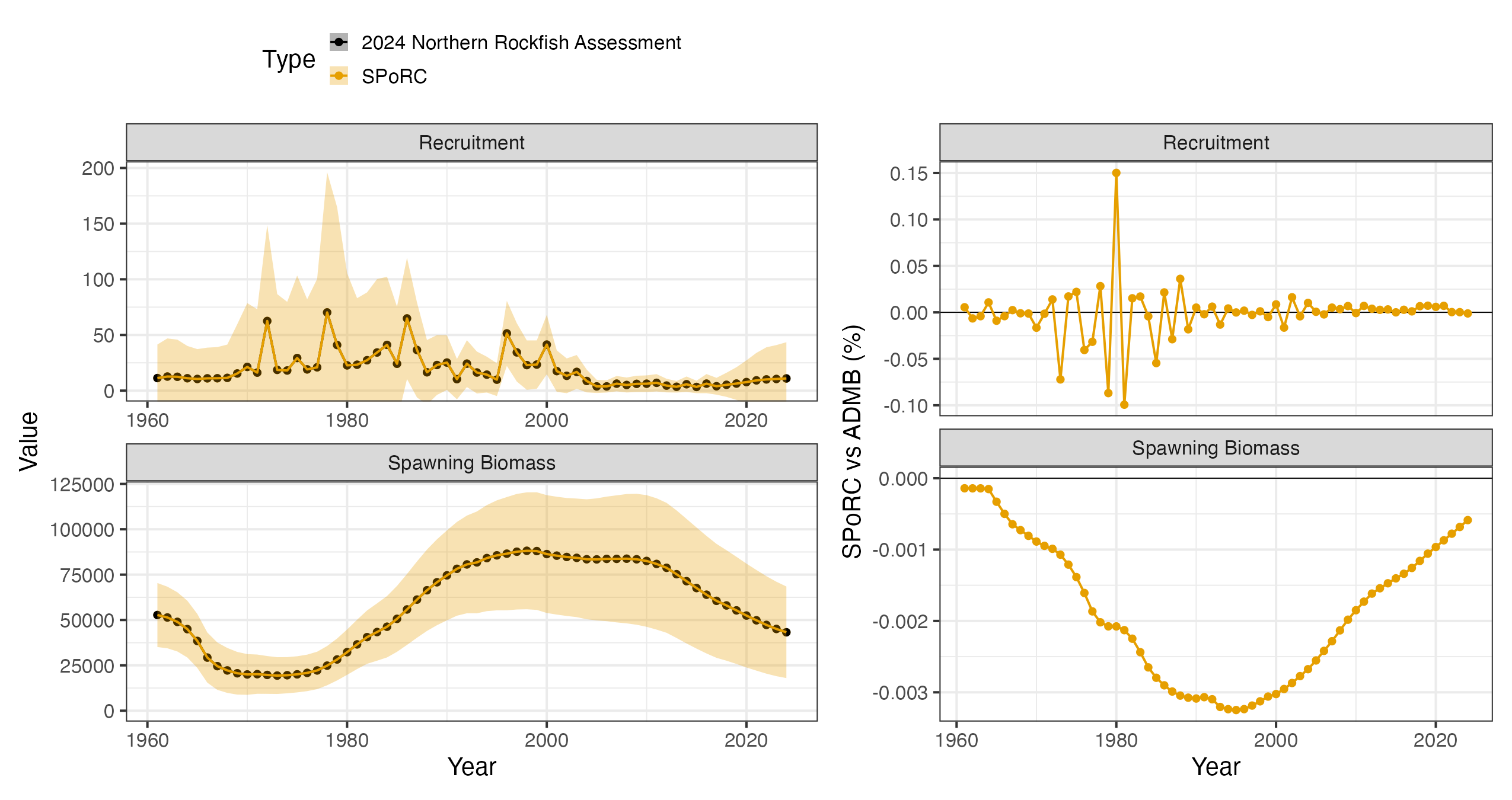
pdHess: TRUESpawning biomass and recruitment are compared below. Because the two series overplot, the percent difference needs its own panel to be readable.
| Quantity | Median difference | Maximum difference |
|---|---|---|
| Spawning biomass | 0.0019 % | 0.0032 % |
| Recruitment | 0.0060 % | 0.150 % |
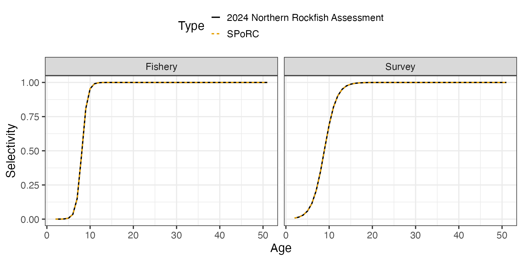
Selectivity is time invariant in both fleets, so a single curve per gear has everything.