North Sea Sandeel (smsR bridge)
Source:vignettes/ah_north_sea_sandeel_case_study.Rmd
ah_north_sea_sandeel_case_study.RmdOverview
This case study bridges smsR, the seasonal assessment
model used for four North Sea sandeel stocks and for sprat, into
SPoRC. The stock is sandeel in area 1r, 1983 to 2021, ages
0 to 4, two seasons, one region and one sex.
smsR is an ICES model rather than one of the US
assessments the other case studies here bridge, and it is built
differently in two ways. Fishing mortality is driven by an observed
effort series rather than estimated year by year, and there are no
composition data at all: catch at age and survey at age enter directly
as lognormal observations, each age with its own catchability and its
own standard deviation.
SPoRC can fit both forms directly, so this reads as an
ordinary specification rather than a translation. Catch at age goes in
through ObsCatchAA and the survey through
ObsSrvIdxAA, with observation error and age-specific
catchability.
| Component | Years | Observations | Likelihood |
|---|---|---|---|
| Catch at age, ages 1 to 4, two seasons | 1983 to 2021 | 286 | Lognormal |
| Dredge survey, ages 0 to 1, season 2 | 2004 to 2021 | 36 | Lognormal |
| RTM survey, ages 1 to 3, season 1 | 2011 to 2020 | 30 | Lognormal |
| Recruitment deviations | 1983 to 2021 | 39 | Lognormal |
Because the model is single region and single sex, the population, region and sex subscripts collapse to one and are dropped from the notation below. The season subscript is retained in the following.
Model dimensions
Two seasons of equal duration, one fishery fleet per season, and the two surveys. A fleet per season is what gives each season its own catch observation error.
input_list <- Setup_Mod_Dim(
  n_pop = 1,
  years = yrs,
  ages = ages,
  lens = NA,
  n_regions = 1,
  n_sexes = 1,
  n_seas = n_seas,
  seasdur = seasdur,
  n_fish_fleets = 2,
  n_srv_fleets = 2,
  verbose = TRUE
)
Recruitment
Recruitment is a mean with annual deviations. smsR
treats its as a hockey stick, but the population dynamics set
recruitment to a free parameter each year and the hockey stick enters
only as a penalty on those deviations, with a weight of 0.05. Spawning
is at the start of season 1 and recruits enter in season 2, one season
later.
input_list <- Setup_Mod_Rec(
  input_list = input_list,
  rec_model = "mean_rec",
  rec_lag = 1,
  spawn_seas = 1,
  t_spawn = 0,
  use_fixed_rec_seas_prop = 1,
  fixed_rec_seas_prop = matrix(c(0, 1), nrow = 1, ncol = n_seas),
  sigmaR_spec = "fix",
  do_rec_bias_ramp = 0,
  init_age_strc = "free",
  equil_init_age_strc = "equil",
  ln_global_R0 = log(2e8)
)

# estiamte these freely so free N per age
input_list$map$ln_InitDevs <- factor(seq_along(input_list$map$ln_InitDevs))
Biological dynamics
smsR stores natural mortality as a free array over age,
year and season, and so does SPoRC. But smsR
stores the mortality accumulated within a season, while
SPoRC stores an instantaneous rate per year and multiplies
it by the season’s duration. The rate is therefore the smsR
number divided by that duration, and with two half-year seasons that is
a factor of two.
Maturity is doubled. SPoRC multiplies spawning biomass
by 0.5 for single sex models, on the reasoning that a single sex model
represents both sexes combined, whereas the smsR ogive
already gives spawning biomass directly. Doubling maturity cancels that
convention and leaves the likelihood untouched. In a two season model
this factor is numerically identical to seasdur[1], which
is a coincidence and not the reason it is there.
# smsR stores its biologicals as [age, year, season]. SPoRC wants
# [pop, region, year, season, age, sex], the same numbers with three dimensions
# of length one, and one more for fleet on the weights a fleet sees.
WAA      <- array(0, dim = c(1, 1, n_yrs, n_seas, n_ages, 1))
MatAA    <- array(0, dim = c(1, 1, n_yrs, n_seas, n_ages, 1))
WAA_fish <- array(0, dim = c(1, 1, n_yrs, n_seas, n_ages, 1, 2))
WAA_srv  <- array(0, dim = c(1, 1, n_yrs, n_seas, n_ages, 1, 2))

for(y in 1:n_yrs) {
  for(seas in 1:n_seas) {
    WAA[1, 1, y, seas, , 1]   = lhs$west[, y, seas]   # stock weight at age
    MatAA[1, 1, y, seas, , 1] = lhs$mat[, y, seas]    # proportion mature at age
    for(f in 1:2) WAA_fish[1, 1, y, seas, , 1, f] = lhs$weca[, y, seas]  # catch weight
    for(k in 1:2) WAA_srv[1, 1, y, seas, , 1, k]  = lhs$west[, y, seas]
  } # end seas loop
} # end y loop

# smsR holds the mortality accumulated within each season. SPoRC parameterizes an
# instantaneous rate per year and multiplies it by the season's duration ...
M_sms <- lhs$M[, 1:n_yrs, ]
natmort <- array(0, dim = c(1, 1, n_yrs, n_seas, n_ages, 1))
for(y in 1:n_yrs) {
  for(seas in 1:n_seas) natmort[1, 1, y, seas, , 1] = M_sms[, y, seas] / seasdur[seas]
} # end y loop

input_list <- Setup_Mod_Biologicals(
  input_list = input_list,
  WAA = WAA,
  WAA_fish = WAA_fish,
  WAA_srv = WAA_srv,
  MatAA = MatAA * 2, # cancels the single sex SSB halving in model dynamics
  fit_lengths = 0,
  M_spec = "fix",
  Fixed_natmort = natmort,
  addtocomp = 1e-5
)
Movement and tagging
Single region, so movement is an identity matrix and no tagging data are used. However, both still have to be declared.
input_list <- Setup_Mod_Movement(
  input_list = input_list,
  use_fixed_movement = 1,
  Fixed_Movement = NA,
  do_recruits_move = 0
)

input_list <- Setup_Mod_Tagging(input_list = input_list, use_conv_fish_tagging = 0)
Catch and fishing mortality
The observation error is coupled by a key matrix over age and fleet,
wjere equal entries share a parameter and NA excludes one.
smsR groups ages 1 and 2 against ages 3 and above,
separately by season, which is four standard deviations. With a fleet
per season that is a plain age by fleet key. Age 0 is never caught, so
it is represented with an NA.
# ages 1-2 and ages 3+ share a standard deviation, separately by season (fleets are defined as season x fishery fleet in this case to allow for seasonal selex)
# the key is age by sex by fleet; this stock is single sex, so the sex dim is 1
sigmaCAA_key <- array(c(NA, 1, 1, 2, 2,
                        NA, 3, 3, 4, 4), dim = c(n_ages, 1, 2))

nocatch <- as.matrix(sandeel_1r$nocatch)
ObsCatchAA <- UseCatchAA <- array(0, dim = c(1, n_yrs, n_seas, n_ages, 1, 2))
for(y in 1:n_yrs) {
  for(s in 1:n_seas) {
    for(a in 2:n_ages) { # age 0 is not fished
      obs = sandeel_1r$Catch[a, y, s]
      if(!is.na(obs) && obs > 0 && nocatch[y, s] == 1) {
        ObsCatchAA[1, y, s, a, 1, s] = obs
        UseCatchAA[1, y, s, a, 1, s] = 1
      }
    } # end a loop
  } # end s loop
} # end y loop

input_list <- Setup_Mod_Catch_and_F(
  input_list = input_list,
  ObsCatch = array(0, dim = c(1, n_yrs, n_seas, 2)),
  UseCatch = array(0, dim = c(1, n_yrs, n_seas, 2)),
  ObsCatchAA = ObsCatchAA,
  UseCatchAA = UseCatchAA,
  sigmaCAA_key = sigmaCAA_key,
  sigmaCAA_spec = "est",
  catch_units = array("abd", dim = c(2)),
  Use_F_pen = 0,
  sigmaC_spec = "fix",
  sigmaF_spec = "fix"
)
A fleet fits the aggregated catch or the catch at age, never both. Supplying both is an error rather than a warning: they are the same information stated twice, and the factorization of an at-age observation into a total and a composition is exact for multinomial counts but not for the lognormal used here.
Effort driven fishing mortality
smsR writes fishing mortality as a seasonal scale times
a blocked age pattern times observed effort:
SPoRC builds it as selectivity times a mean and a
deviation:
where
| Symbol | Meaning | Here |
|---|---|---|
| age | 0 to 4 | |
| year | 1983 to 2021 | |
| season | 1 or 2, each half a year | |
| fishery fleet | 1 or 2; fleet fishes season alone | |
| the selectivity block year falls in | block 1 is 1983-1998, block 2 is 1999-2021 | |
| fishing mortality at age | what the two models have to agree on | |
| observed effort, a data series | median about 2100 | |
| fishery selectivity at age, constant within a block | 6 estimated values | |
log of the fleet’s scale, ln_F_mean
|
2 estimated values | |
fishing mortality deviation, ln_F_devs
|
kept at , not estimated |
Setting and holding it there makes the two identical, because .
Written that way is a catchability. This is basically the effort model,
with scaling effort into fishing mortality and spreading it over ages. The deviations hold data rather than estimated quantities, so they are mapped off.
effort <- sandeel_1r$effort
dev_dim <- dim(input_list$par$ln_F_devs)
ln_F_devs <- array(0, dim = dev_dim)
for(y in 1:dev_dim[2]) {
  for(seas in 1:dev_dim[3]) ln_F_devs[1, y, seas, ] = log(effort[y, seas])
} # end y loop

input_list$par$ln_F_devs <- ln_F_devs
input_list$map$ln_F_devs <- factor(array(NA, dim = dev_dim))
input_list$par$ln_F_mean[] <- -5 # starting values ... for 'q'
Fishery selectivity
smsR zeroes fishing on age 0 through its age selectivity
and shares selectivity across ages 3 and above. Both are set through the
selectivity map: age 0 kept at a value giving zero selection, and ages 3
and 4 sharing a parameter, in each of the two blocks.
Also, smsR writes its age pattern relative to a
reference: ages 3 and above are the top of the curve and the younger
ages are ratios to them, with the overall level living in the seasonal
scale. To mimick this, we use a free non-parametric selectivity curve on
log scale, without standardization:
with
the selectivity at age
in block
and
the estimated parameter behind it. Because nothing is divided out,
is a selectivity of exactly one and a large negative
is a selectivity of zero, so both of the things smsR fixes
are set by fixing
rather than by any extra routines:
The first line is age 0, never fished. The second is block one’s reference, kept at one so the level of fishing stays in . Everything else is estimated, and what it estimates is a ratio to that reference. Putting it together with the effort model above, fishing mortality at age is
There is no fishery index here, so that data source is declared empty.
empty_fish <- list(
  ObsFishIdx = array(NA, dim = c(1, n_yrs, n_seas, 2)),
  ObsFishIdx_SE = array(NA, dim = c(1, n_yrs, n_seas, 2)),
  UseFishIdx = array(0, dim = c(1, n_yrs, n_seas, 2)),
  ObsFishAgeComps = array(0, dim = c(1, n_yrs, n_seas, n_ages, 1, 2)),
  UseFishAgeComps = array(0, dim = c(1, n_yrs, n_seas, 2)),
  ISS_FishAgeComps = array(0, dim = c(1, n_yrs, n_seas, 1, 2)),
  ObsFishLenComps = array(0, dim = c(1, n_yrs, n_seas, 1, 1, 2)),
  UseFishLenComps = array(0, dim = c(1, n_yrs, n_seas, 2)),
  ISS_FishLenComps = array(0, dim = c(1, n_yrs, n_seas, 1, 2)))

input_list <- do.call(Setup_Mod_FishIdx_and_Comps, c(
  list(input_list = input_list,
       fish_idx_type = rep("none", 2),
       FishAgeComps_LikeType = rep("none", 2),
       FishLenComps_LikeType = rep("none", 2),
       FishAgeComps_Type = c("agg_Year_1-terminal_Fleet_1", "agg_Year_1-terminal_Fleet_2"),
       FishLenComps_Type = c("agg_Year_1-terminal_Fleet_1", "agg_Year_1-terminal_Fleet_2")),
  empty_fish))

# non-parametric selectivity at age, two blocks, ages 3 and 4 grouped
input_list <- Setup_Mod_Fishsel_and_Q(
  input_list = input_list,
  cont_tv_fish_sel = c("none_Fleet_1", "none_Fleet_2"),
  fish_sel_blocks = c("Block_1_Year_1-16_Fleet_1", "Block_2_Year_17-terminal_Fleet_1",
                      "Block_1_Year_1-16_Fleet_2", "Block_2_Year_17-terminal_Fleet_2"),
  fish_sel_model = c("nonparfree_Fleet_1", "nonparfree_Fleet_2"),
  fish_q_blocks = c("none_Fleet_1", "none_Fleet_2"),
  fish_sel_nonpar_est_bins = rep(list(list(list(1, 2, 3, c(4, 5)), list(1, 2, 3, c(4, 5)))), 2),
  fish_fixed_sel_pars_spec = rep("est_all", 2),
  fish_q_spec = rep("fix", 2))

# Fishery selectivity is one value per age, per block, shared by the two season
# fleets because smsR's age pattern does not vary by season.
sel_par <- rbind(block_1 = c(NA, 1L, 2L, NA, NA),
                 block_2 = c(NA, 3L, 4L, 5L, 5L))

# fish_fixed_sel_pars is [region, age, block, sex, fleet]. for "nonparfree" a
# value of 0 is a selectivity of one, and -10 is a selectivity of zero.
sel_start <- input_list$par$fish_fixed_sel_pars
sel_map <- array(NA_integer_, dim = dim(sel_start))
sel_start[1, , , 1, ] <- 0
sel_start[1, 1, , 1, ] <- -10                # age 0, never fished
for(b in 1:2) {
  for(f in 1:2) sel_map[1, , b, 1, f] <- sel_par[b, ]
} # end b loop

input_list$par$fish_fixed_sel_pars <- sel_start
input_list$map$fish_fixed_sel_pars <- factor(sel_map)
Survey index
smsR fits each survey age as its own lognormal series
with its own catchability: the Dredge over ages 0 and 1 in season 2, the
RTM over ages 1 to 3 in season 1, five catchabilities in total.
SPoRC does that through ObsSrvIdxAA.
Those five catchabilities do not need a parameter of their own.
smsR predicts a survey observation as
with
the index at age,
a catchability estimated separately at every age
of survey
,
the numbers at age,
how far into its season the survey happens, and
total mortality. SPoRC predicts the same thing as
which is the same equation with the age multiplier called selectivity
instead of catchability. A free catchability per age and a selectivity
estimated at age are one quantity written two ways, and estimating both
would be estimating it twice. So the age shape goes in selectivity,
again through "nonparfree", and there is no age-specific
at all:
srv_sel_nonpar_est_bins then does the grouping a
catchability key would, and an age left out of the list gets no
parameter, which is what an age a survey never sees wants.
# the Dredge runs in season 2 over ages 0-1, the RTM in season 1 over ages 1-3
srv_ages <- list(0:1, 1:3)
srv_seas <- c(2, 1)

ObsSrvIdxAA <- UseSrvIdxAA <- array(0, dim = c(1, n_yrs, n_seas, n_ages, 1, 2))
for(k in 1:2) {
  for(a in srv_ages[[k]]) {
    arow = which(ages == a)
    for(y in 1:n_yrs) {
      obs = sandeel_1r$survey[arow, y, k]
      if(!is.na(obs) && obs > 0) {
        ObsSrvIdxAA[1, y, srv_seas[k], arow, 1, k] = obs
        UseSrvIdxAA[1, y, srv_seas[k], arow, 1, k] = 1
      }
    } # end y loop
  } # end a loop
} # end k loop

# smsR groups its survey standard deviations by age within a survey
sigmaSrvIdxAA_key <- array(NA, dim = c(n_ages, 1, 2))
sigmaSrvIdxAA_key[2, 1, 1] <- 1
sigmaSrvIdxAA_key[2, 1, 2] <- 2
sigmaSrvIdxAA_key[3:4, 1, 2] <- 3

# The Dredge's age-0 value is kept rather than estimated. Age 0 appears in this
# one index and nowhere else, and the recruitment deviations are free, so they
# fit it exactly: the residual goes to zero and the likelihood is unbounded.
sigmaSrvIdxAA_start <- array(log(0.5), dim = c(n_ages, 1, 2))
sigmaSrvIdxAA_start[1, 1, 1] <- log(0.4052)   # smsR's own value

empty_srv <- list(
  ObsSrvAgeComps = array(0, dim = c(1, n_yrs, n_seas, n_ages, 1, 2)),
  UseSrvAgeComps = array(0, dim = c(1, n_yrs, n_seas, 2)),
  ISS_SrvAgeComps = array(0, dim = c(1, n_yrs, n_seas, 1, 2)),
  ObsSrvLenComps = array(0, dim = c(1, n_yrs, n_seas, 1, 1, 2)),
  UseSrvLenComps = array(0, dim = c(1, n_yrs, n_seas, 2)),
  ISS_SrvLenComps = array(0, dim = c(1, n_yrs, n_seas, 1, 2)))

input_list <- do.call(Setup_Mod_SrvIdx_and_Comps, c(
  list(input_list = input_list,
       ObsSrvIdx = array(NA, dim = c(1, n_yrs, n_seas, 2)),
       ObsSrvIdx_SE = array(0, dim = c(1, n_yrs, n_seas, 2)),
       UseSrvIdx = array(0, dim = c(1, n_yrs, n_seas, 2)),
       ObsSrvIdxAA = ObsSrvIdxAA,
       UseSrvIdxAA = UseSrvIdxAA,
       sigmaSrvIdxAA_key = sigmaSrvIdxAA_key,
       sigmaSrvIdxAA_spec = "est",
       ln_sigmaSrvIdxAA = sigmaSrvIdxAA_start,
       srv_idx_type = rep("abd", 2),
       SrvAgeComps_LikeType = rep("none", 2),
       SrvLenComps_LikeType = rep("none", 2),
       SrvAgeComps_Type = c("agg_Year_1-terminal_Fleet_1", "agg_Year_1-terminal_Fleet_2"),
       SrvLenComps_Type = c("agg_Year_1-terminal_Fleet_1", "agg_Year_1-terminal_Fleet_2")),
  empty_srv))

# each survey enters at its own point in its own season
t_srv <- array(0, dim = c(1, n_seas, 2))
for(k in 1:2) t_srv[1, srv_seas[k], k] <- c(0.75, 0)[k]

input_list <- Setup_Mod_Srvsel_and_Q(
  input_list = input_list,
  cont_tv_srv_sel = c("none_Fleet_1", "none_Fleet_2"),
  srv_sel_blocks = c("none_Fleet_1", "none_Fleet_2"),
  srv_sel_model = c("nonparfree_Fleet_1", "nonparfree_Fleet_2"),
  srv_q_blocks = c("none_Fleet_1", "none_Fleet_2"),
  # one value per age each survey observes: the Dredge ages 0-1, the RTM ages 1-3
  srv_sel_nonpar_est_bins = list(list(list(1, 2)), list(list(2, 3, 4))),
  srv_fixed_sel_pars_spec = rep("est_all", 2),
  srv_q_spec = rep("fix", 2),
  t_srv = t_srv)
Weighting
No data-weighting is done in this section, so everything is set at 1.
input_list <- Setup_Mod_Weighting(
  input_list = input_list,
  Wt_Catch = 1, Wt_FishIdx = 0, Wt_SrvIdx = 1, Wt_Rec = 1, Wt_F = 1, Wt_Tagging = 0,
  Wt_FishAgeComps = array(0, dim = c(1, n_yrs, n_seas, 1, 2)),
  Wt_FishLenComps = array(0, dim = c(1, n_yrs, n_seas, 1, 2)),
  Wt_SrvAgeComps = array(0, dim = c(1, n_yrs, n_seas, 1, 2)),
  Wt_SrvLenComps = array(0, dim = c(1, n_yrs, n_seas, 1, 2)))
Fitting
input_list$par$ln_sigmaR[] <- log(1)
est <- fit_model(input_list$data, input_list$par, input_list$map,
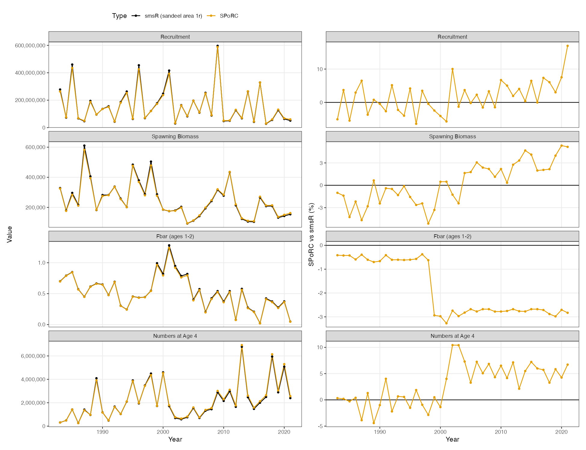
random = NULL, newton_loops = 3, silent = FALSE)| Quantity | Correlation | Median annual difference | Largest annual difference |
|---|---|---|---|
| Spawning biomass | 0.9989 | 2.18 % | 5.32 % |
| Recruitment | 0.9993 | 3.70 % | 16.97 % |
| Numbers at ages 1 to 4 | 0.9985 to 0.9994 | 3.58 to 4.22 % | 10.02 to 15.26 % |
| Fbar, ages 1 and 2 | 0.9997 | 2.68 % | 3.27 % |
Seeded at smsR’s own MLE rather than refitted, the
population dynamics agree to 4e-11 %, so the table shows where the two
likelihoods disagree, not where the population models do. The biggest
recruitment differences land in the years the smsR hockey
stick penalty pulls hardest, the structural difference noted below.