One-Step-Ahead (OSA) Residuals • SPoRC

Raw (Pearson) residuals from compositional, count, and index data can be difficult to interpret given that multinomial/Dirichlet-multinomial proportions are correlated within a year (they must sum to one), tag recapture counts are correlated across cohorts and liberty classes, and even continuous index/catch observations are correlated through the shared state variables (abundance, selectivity) that predict them. One-step-ahead (OSA) residuals remove these correlations by computing, for each observation, the residual of its predictive distribution conditional on all previous observations. Thus, this conditioning should theoretically remove all associated correlaitons and the result should behave like iid standard normal deviates if the model is correctly specified, making standard diagnostics (QQ-plots, SDNR, autocorrelation) meaningful.

SPoRC computes OSA residuals through a single entry point, get_osa(), which supports two independent computation modes and every major data type in the package:

Data type	`get_osa()` argument	Family
Age/length compositions	`comp_source = "FishAge"/"FishLen"/"SrvAge"/"SrvLen"`	discrete (multinomial/DM) or continuous (logistic-normal)
Population-specific compositions	add `pop = TRUE`	same as above
Discard compositions	add `discard = TRUE`	same as above
Conventional tag recoveries	`tag = TRUE`	discrete (count or comp-conditioned)
Catch	`index_source = "Catch"`	continuous (log-normal)
Discards	`index_source = "Discard"`	continuous (log-normal)
Fishery index	`index_source = "FishIdx"`	continuous (log-normal)
Survey index	`index_source = "SrvIdx"`	continuous (log-normal)
Any index source, population-specific	add `pop = TRUE`	continuous (log-normal)

Every get_osa() call returns a list with a single element, res, a data frame of residuals that can be passed directly to plot_resids(), which produces a QQ-plot (with an SDNR annotation) and a second diagnostic plot (a bubble plot for compositions/tags, or a residual-vs-year plot for index-type data).

Two computation modes

External (post-hoc), get_osa(obs_mat = , exp_mat = , N = , ...). Works with any fitted model, no special setup required. Observed/expected arrays (typically pulled from get_comp_prop()) are handed to the compResidual package, which builds a small TMB model and computes OSA residuals independently of how the main model was fit.

Internal (model-based), get_osa(model = , data = , ...). Internal OSA is only required for composition data and conventional tagging data. Catch and abundance index observations (Catch/Discard/FishIdx/SrvIdx) are handled automatically through the model likelihood and do not require any additional setup. To obtain internal OSA residuals for composition and/or tagging data, the model must be re-fit with do_internal_comp_osa = TRUE and/or do_internal_conv_tag_osa = TRUE in Setup_Mod_Dim(). These options wrap the relevant observations in RTMB::OBS() at the point they enter the model likelihood, allowing RTMB::oneStepPredict() to operate directly on the fitted model object.

When do_internal_comp_osa = TRUE, the observed composition proportions (Obs) are internally converted to integer counts (e.g., ISS × Wt × Obs) before entering the multinomial or Dirichlet-multinomial likelihood, since these likelihoods are defined on count data. The resulting counts are rounded to the nearest integer. This generally has negligible impact when the effective sample size (e.g., ISS × Wt) is large, but users should be aware that it can alter the likelihood relative to using continuous proportions. This is particularly relevant when applying Francis or other composition reweighting methods, since the weighted effective sample size determines the counts supplied to the likelihood.

It is strongly recommended that the composition weighting factors (Wt_*) remain at their default values when using internal OSA. These weights are applied after the likelihood contribution has been calculated rather than being passed directly into dnorm(), dmultinom(), ddirmult(), or other likelihood functions. Consequently, they are not incorporated into the one-step-ahead predictive distribution and can produce OSA diagnostics that are difficult to interpret or inconsistent with the fitted objective function.

Both modes are demonstrated below on the same real dataset (single-region GOA Dusky Rockfish) so the two can be compared directly, plus a simulated multi-population, tagging-enabled model for the internal-only data types.

library(SPoRC)
library(tidyverse)
data("sgl_rg_dusky_data")

External OSA residuals

Any already-fitted model works. get_comp_prop() extracts observed/expected proportions from the model report, and get_osa() (no model= argument) computes OSA residuals from those arrays via compResidual.

input_list <- Setup_Mod_Dim(
  years = sgl_rg_dusky_data$years,
  ages = sgl_rg_dusky_data$mod_ages,
  lens = sgl_rg_dusky_data$lens,
  n_regions = sgl_rg_dusky_data$n_regions,
  n_sexes = sgl_rg_dusky_data$n_sexes,
  n_fish_fleets = sgl_rg_dusky_data$n_fish_fleets,
  n_srv_fleets = sgl_rg_dusky_data$n_srv_fleets,
  bias_correct_pe = "none", # the assessment corrects neither recruitment nor the initial ages
  verbose = FALSE
  # note: do_internal_comp_osa is NOT set here which is not needed for the
  # external path
)

input_list <- Setup_Mod_Rec(
  input_list = input_list,
  sigmaR_switch = 1,
  ln_sigmaR = array(-0.1068576, dim = c(2, input_list$data$n_pop, input_list$data$n_regions)),
  rec_model = "mean_rec",
  sigmaR_spec = "fix",
  init_age_strc = 1,
  ln_global_R0 = log(2.7),
  t_spawn = sgl_rg_dusky_data$spwn_month
)

input_list <- Setup_Mod_Biologicals(
  input_list = input_list,
  WAA = sgl_rg_dusky_data$waa_arr,
  MatAA = sgl_rg_dusky_data$mataa_arr,
  fit_lengths = 1,
  SizeAgeTrans = sgl_rg_dusky_data$sizeage,
  AgeingError = sgl_rg_dusky_data$age_error_matrix,
  M_spec = "fix",
  Fixed_natmort = sgl_rg_dusky_data$fix_natmort,
  addtocomp = 0.00001
)

input_list <- Setup_Mod_Movement(
  input_list = input_list,
  use_fixed_movement = 1,
  Fixed_Movement = NA,
  do_recruits_move = 0
)

input_list <- Setup_Mod_Tagging(input_list = input_list, use_conv_fish_tagging = 0)

input_list <- Setup_Mod_Catch_and_F(
  input_list = input_list,
  ObsCatch = sgl_rg_dusky_data$ObsCatch,
  UseCatch = sgl_rg_dusky_data$UseCatch,
  Use_F_pen = 1,
  sigmaC_spec = "fix",
  Catch_Constant = 0.00001,
  ln_sigmaC = array(log(sqrt(1 / (2 * c(rep(2, 15), rep(50, 33))))), dim = c(input_list$data$n_regions, length(input_list$data$years),
                                              input_list$data$n_seas, input_list$data$n_fish_fleets)),
  ln_sigmaF = array(log(sqrt(1 / 4)), dim = c(input_list$data$n_regions, input_list$data$n_seas,
                                              input_list$data$n_fish_fleets))
)

input_list <- Setup_Mod_FishIdx_and_Comps(
  input_list = input_list,
  ObsFishIdx = sgl_rg_dusky_data$ObsFishIdx,
  ObsFishIdx_SE = sgl_rg_dusky_data$ObsFishIdx_SE,
  UseFishIdx = sgl_rg_dusky_data$UseFishIdx,
  ObsFishAgeComps = sgl_rg_dusky_data$ObsFishAgeComps,
  UseFishAgeComps = sgl_rg_dusky_data$UseFishAgeComps,
  ISS_FishAgeComps = sgl_rg_dusky_data$ISS_FishAgeComps,
  ObsFishLenComps = sgl_rg_dusky_data$ObsFishLenComps,
  UseFishLenComps = sgl_rg_dusky_data$UseFishLenComps,
  ISS_FishLenComps = sgl_rg_dusky_data$ISS_FishLenComps,
  fish_idx_type = c("none"),
  FishAgeComps_LikeType = c("Multinomial"),
  FishLenComps_LikeType = c("Multinomial"),
  FishAgeComps_Type = c("agg_Year_1-terminal_Fleet_1"),
  FishLenComps_Type = c("agg_Year_1-terminal_Fleet_1")
)

input_list <- Setup_Mod_SrvIdx_and_Comps(
  input_list = input_list,
  ObsSrvIdx = sgl_rg_dusky_data$ObsSrvIdx,
  ObsSrvIdx_SE = (sgl_rg_dusky_data$ObsSrvIdx_SE / sgl_rg_dusky_data$ObsSrvIdx) / sqrt(1.66),
  UseSrvIdx = sgl_rg_dusky_data$UseSrvIdx,
  ObsSrvAgeComps = sgl_rg_dusky_data$ObsSrvAgeComps,
  ISS_SrvAgeComps = sgl_rg_dusky_data$ISS_SrvAgeComps,
  UseSrvAgeComps = sgl_rg_dusky_data$UseSrvAgeComps,
  ObsSrvLenComps = sgl_rg_dusky_data$ObsSrvLenComps,
  UseSrvLenComps = sgl_rg_dusky_data$UseSrvLenComps,
  ISS_SrvLenComps = sgl_rg_dusky_data$ISS_SrvLenComps,
  srv_idx_type = c("biom"),
  SrvAgeComps_LikeType = c("Multinomial"),
  SrvLenComps_LikeType = c("Multinomial"),
  SrvAgeComps_Type = c("agg_Year_1-terminal_Fleet_1"),
  SrvLenComps_Type = c("agg_Year_1-terminal_Fleet_1")
)

input_list <- Setup_Mod_Fishsel_and_Q(
  input_list = input_list,
  cont_tv_fish_sel = c("none_Fleet_1"),
  fish_sel_blocks = c("none_Fleet_1"),
  fish_sel_model = c("logist2_Fleet_1"),
  fish_q_blocks = c("none_Fleet_1"),
  fish_fixed_sel_pars_spec = c("est_all"),
  fish_q_spec = c("fix")
)

srv_q_prior <- data.frame(region = 1, block = 1, fleet = 1, mu = 1, sd = 0.447213595)

input_list <- Setup_Mod_Srvsel_and_Q(
  input_list = input_list,
  cont_tv_srv_sel = c("none_Fleet_1"),
  srv_sel_blocks = c("none_Fleet_1"),
  srv_sel_model = c("logist2_Fleet_1"),
  srv_q_blocks = c("none_Fleet_1"),
  srv_fixed_sel_pars_spec = c("est_all"),
  srv_q_spec = c("est_all"),
  Use_srv_q_prior = 1,
  srv_q_prior = srv_q_prior,
  t_srv = array(0, dim = c(input_list$data$n_regions, input_list$data$n_seas, input_list$data$n_srv_fleets))
)

input_list <- Setup_Mod_Weighting(
  input_list
)


model <- fit_model(input_list$data, input_list$par, input_list$map,
                   random = NULL, newton_loops = 3, silent = TRUE)

# Modeled ages span sgl_rg_dusky_data$mod_ages (4:33, 30 ages), but observed
# fishery/survey age compositions only report ages 4:30 (27 bins, an
# ageing-error offset), comp bin labels use the *observed* bin range.
obs_age_bins <- 4:30

comp_prop <- get_comp_prop(input_list$data, model$rep,
                           age_labels = obs_age_bins,
                           len_labels = sgl_rg_dusky_data$lens,
                           year_labels = sgl_rg_dusky_data$years)

fishages_ext <- get_osa(
  obs_mat = comp_prop$Obs_FishAge_mat,
  exp_mat = comp_prop$Pred_FishAge_mat,
  N = input_list$data$ISS_FishAgeComps[1, which(input_list$data$UseFishAgeComps[,,1,1] == 1), 1, 1, 1] *
    unique(input_list$data$Wt_FishAgeComps[1, which(input_list$data$UseFishAgeComps[,,1,1] == 1), 1, , 1]),
  years = which(input_list$data$UseFishAgeComps[,,1,1] == 1),
  fleet = 1,
  bins = obs_age_bins,
  seas = 1,
  comp_type = 0, # aggregated across sex/region
  bin_label = "Ages"
)

resid_ext <- plot_resids(fishages_ext)
resid_ext[[1]] # QQ-plot with SDNR
resid_ext[[2]] # bubble plot of residuals by year x age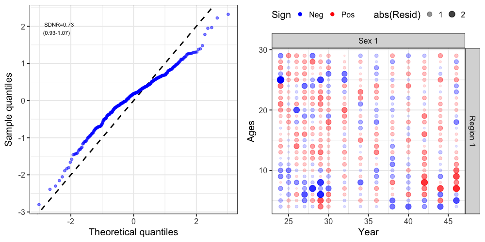

Internal OSA residuals

Composition and index data

Refitting the same Dusky Rockfish model with do_internal_comp_osa = TRUE switches on RTMB::OBS() tracking for every composition source, plus (unconditionally, no extra flag needed) Catch, Discard, FishIdx, and SrvIdx. get_osa() is then called with model =/data = instead of obs_mat =/exp_mat =.

input_list <- Setup_Mod_Dim(
  years = sgl_rg_dusky_data$years,
  ages = sgl_rg_dusky_data$mod_ages,
  lens = sgl_rg_dusky_data$lens,
  n_regions = sgl_rg_dusky_data$n_regions,
  n_sexes = sgl_rg_dusky_data$n_sexes,
  n_fish_fleets = sgl_rg_dusky_data$n_fish_fleets,
  n_srv_fleets = sgl_rg_dusky_data$n_srv_fleets,
  bias_correct_pe = "none", # the assessment corrects neither recruitment nor the initial ages
  verbose = FALSE,
  do_internal_comp_osa = TRUE # the only change needed vs. the external setup
)

input_list <- Setup_Mod_Rec(
  input_list = input_list,
  sigmaR_switch = 1,
  ln_sigmaR = array(-0.1068576, dim = c(2, input_list$data$n_pop, input_list$data$n_regions)),
  rec_model = "mean_rec",
  sigmaR_spec = "fix",
  init_age_strc = 1,
  ln_global_R0 = log(2.7),
  t_spawn = sgl_rg_dusky_data$spwn_month
)

input_list <- Setup_Mod_Biologicals(
  input_list = input_list,
  WAA = sgl_rg_dusky_data$waa_arr,
  MatAA = sgl_rg_dusky_data$mataa_arr,
  fit_lengths = 1,
  SizeAgeTrans = sgl_rg_dusky_data$sizeage,
  AgeingError = sgl_rg_dusky_data$age_error_matrix,
  M_spec = "fix",
  Fixed_natmort = sgl_rg_dusky_data$fix_natmort,
  addtocomp = 0.00001
)

input_list <- Setup_Mod_Movement(
  input_list = input_list,
  use_fixed_movement = 1,
  Fixed_Movement = NA,
  do_recruits_move = 0
)

input_list <- Setup_Mod_Tagging(input_list = input_list, use_conv_fish_tagging = 0)

input_list <- Setup_Mod_Catch_and_F(
  input_list = input_list,
  ObsCatch = sgl_rg_dusky_data$ObsCatch,
  UseCatch = sgl_rg_dusky_data$UseCatch,
  Use_F_pen = 1,
  sigmaC_spec = "fix",
  Catch_Constant = 0.00001,
  ln_sigmaC = array(log(sqrt(1 / (2 * c(rep(2, 15), rep(50, 33))))), dim = c(input_list$data$n_regions, length(input_list$data$years),
                                              input_list$data$n_seas, input_list$data$n_fish_fleets)),
  ln_sigmaF = array(log(sqrt(1 / 4)), dim = c(input_list$data$n_regions, input_list$data$n_seas,
                                              input_list$data$n_fish_fleets))
)

input_list <- Setup_Mod_FishIdx_and_Comps(
  input_list = input_list,
  ObsFishIdx = sgl_rg_dusky_data$ObsFishIdx,
  ObsFishIdx_SE = sgl_rg_dusky_data$ObsFishIdx_SE,
  UseFishIdx = sgl_rg_dusky_data$UseFishIdx,
  ObsFishAgeComps = sgl_rg_dusky_data$ObsFishAgeComps,
  UseFishAgeComps = sgl_rg_dusky_data$UseFishAgeComps,
  ISS_FishAgeComps = sgl_rg_dusky_data$ISS_FishAgeComps,
  ObsFishLenComps = sgl_rg_dusky_data$ObsFishLenComps,
  UseFishLenComps = sgl_rg_dusky_data$UseFishLenComps,
  ISS_FishLenComps = sgl_rg_dusky_data$ISS_FishLenComps,
  fish_idx_type = c("none"),
  FishAgeComps_LikeType = c("Multinomial"),
  FishLenComps_LikeType = c("Multinomial"),
  FishAgeComps_Type = c("agg_Year_1-terminal_Fleet_1"),
  FishLenComps_Type = c("agg_Year_1-terminal_Fleet_1")
)

input_list <- Setup_Mod_SrvIdx_and_Comps(
  input_list = input_list,
  ObsSrvIdx = sgl_rg_dusky_data$ObsSrvIdx,
  ObsSrvIdx_SE = (sgl_rg_dusky_data$ObsSrvIdx_SE / sgl_rg_dusky_data$ObsSrvIdx) / sqrt(1.66),
  UseSrvIdx = sgl_rg_dusky_data$UseSrvIdx,
  ObsSrvAgeComps = sgl_rg_dusky_data$ObsSrvAgeComps,
  ISS_SrvAgeComps = sgl_rg_dusky_data$ISS_SrvAgeComps,
  UseSrvAgeComps = sgl_rg_dusky_data$UseSrvAgeComps,
  ObsSrvLenComps = sgl_rg_dusky_data$ObsSrvLenComps,
  UseSrvLenComps = sgl_rg_dusky_data$UseSrvLenComps,
  ISS_SrvLenComps = sgl_rg_dusky_data$ISS_SrvLenComps,
  srv_idx_type = c("biom"),
  SrvAgeComps_LikeType = c("Multinomial"),
  SrvLenComps_LikeType = c("Multinomial"),
  SrvAgeComps_Type = c("agg_Year_1-terminal_Fleet_1"),
  SrvLenComps_Type = c("agg_Year_1-terminal_Fleet_1")
)

input_list <- Setup_Mod_Fishsel_and_Q(
  input_list = input_list,
  cont_tv_fish_sel = c("none_Fleet_1"),
  fish_sel_blocks = c("none_Fleet_1"),
  fish_sel_model = c("logist2_Fleet_1"),
  fish_q_blocks = c("none_Fleet_1"),
  fish_fixed_sel_pars_spec = c("est_all"),
  fish_q_spec = c("fix")
)

srv_q_prior <- data.frame(region = 1, block = 1, fleet = 1, mu = 1, sd = 0.447213595)

input_list <- Setup_Mod_Srvsel_and_Q(
  input_list = input_list,
  cont_tv_srv_sel = c("none_Fleet_1"),
  srv_sel_blocks = c("none_Fleet_1"),
  srv_sel_model = c("logist2_Fleet_1"),
  srv_q_blocks = c("none_Fleet_1"),
  srv_fixed_sel_pars_spec = c("est_all"),
  srv_q_spec = c("est_all"),
  Use_srv_q_prior = 1,
  srv_q_prior = srv_q_prior,
  t_srv = array(0, dim = c(input_list$data$n_regions, input_list$data$n_seas, input_list$data$n_srv_fleets))
)

input_list <- Setup_Mod_Weighting(
  input_list
)

model <- fit_model(input_list$data, input_list$par, input_list$map,
                   random = NULL, newton_loops = 3, silent = TRUE)

# Composition OSA: comp_source identifies the data source, family whether
# the fitted likelihood for that source is discrete (multinomial/DM) or
# continuous (logistic-normal)
fishages_int <- get_osa(model = model, data = input_list$data,
                        comp_source = "FishAge", family = "discrete",
                        bins = obs_age_bins, bin_label = "Ages")
resid_int <- plot_resids(fishages_int)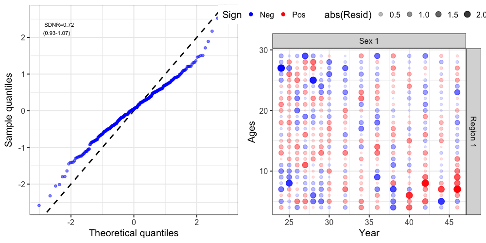

Index-type sources use index_source instead of comp_source/family, there is no likelihood-family choice to make, since these are always continuous log-normal observations (currently), and no bins/bin_label since there’s no bin dimension. plot_resids() returns a QQ-plot paired with a residual-vs-year plot instead of a bubble plot. The residuals for catch appear visually ‘odd’ likely due to a change in the variance of the distribution between early and late periods, reflecting a change in catch observations for Dusky rockfish during these periods (i.e., catches were recorded a a mix of different rockfish species earlier in the time series, and the variance is adjusted to reflect increased uncertainty in the catch observation).

catch_int  <- get_osa(model = model, data = input_list$data, index_source = "Catch")
srvidx_int <- get_osa(model = model, data = input_list$data, index_source = "SrvIdx")
# index_source = "Discard"/"FishIdx" follow the identical interface (omitted
# here ... this Dusky Rockfish case study sets fish_idx_type = "none" and
# doesn't model discards, so those sources have no data to show)

resid_catch  <- plot_resids(catch_int)
resid_srvidx <- plot_resids(srvidx_int)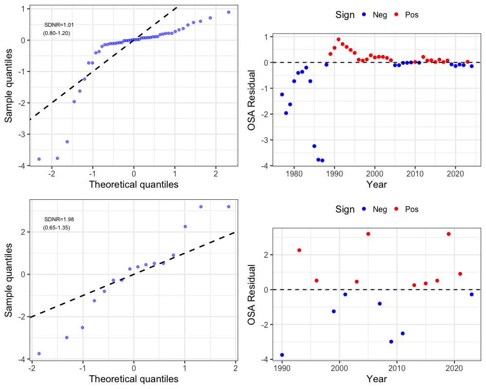

Age-disaggregated observations

Catch at age, discards at age, and the survey index at age all support one-step-ahead residuals. Pass the at-age name as index_source. This case study fits aggregated catch, so the call below is for a model that fits catch at age:

osa <- get_osa(model = model, data = input_list$data, index_source = "CatchAA")
plot_resids(osa)

Valid at-age sources are "CatchAA", "DiscardAA" and "SrvIdxAA", each with a pop = TRUE variant. The returned data frame has an extra age column, which the residual plots facet on.

Population-specific and tagging data

Population-specific composition/index residuals (pop = TRUE) and conventional tag recovery residuals (tag = TRUE) require the model to actually have population-specific and/or tagging data, so this section switches to a simulated 3-population, 2-region, 2-season model with natal homing movement and conventional tagging, fit with both do_internal_comp_osa = TRUE and do_internal_conv_tag_osa = TRUE. The following code chunk is purely for demonstration purposes.

input_pop <- Setup_Mod_Dim(
  years = 1:sim_obj$n_years, ages = 1:sim_obj$n_ages, lens = sim_obj$n_lens,
  n_regions = sim_obj$n_regions, n_sexes = sim_obj$n_sexes,
  n_fish_fleets = sim_obj$n_fish_fleets, n_srv_fleets = sim_obj$n_srv_fleets,
  n_seas = sim_obj$n_seas, n_pop = sim_obj$n_pop,
  natal_region = c(1, 1, 2), verbose = FALSE,
  do_internal_comp_osa = TRUE,
  do_internal_conv_tag_osa = TRUE
)

model_pop <- fit_model(input_pop$data, input_pop$par, input_pop$map,
                       random = NULL, newton_loops = 3, silent = TRUE)

Population-specific composition OSA (pop = TRUE, joint-sex in this example):

comp_pop <- get_osa(model = model_pop, data = input_pop$data, comp_source = "FishAge",
                    pop = TRUE, family = "discrete", bins = input_pop$data$ages, bin_label = "Ages")
resid_comp_pop <- plot_resids(comp_pop)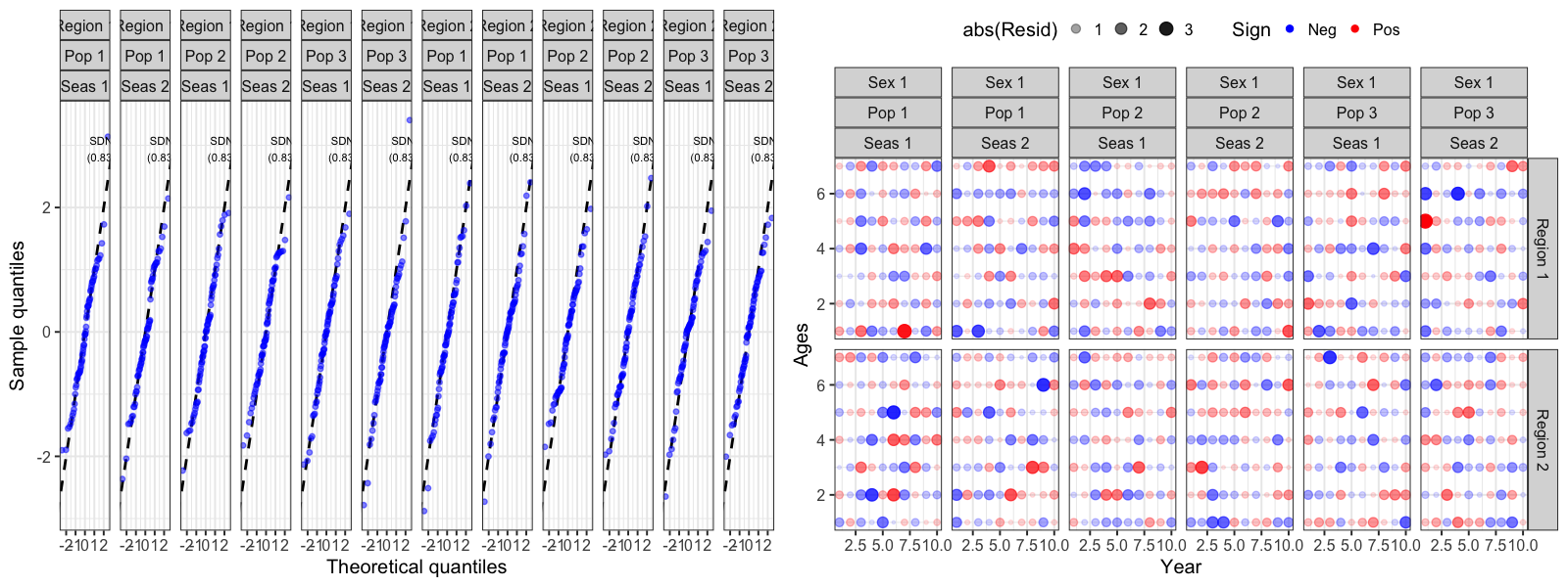

Conventional tag recovery OSA (tag = TRUE), faceted by region, recovery season, fleet, and movement/tag pooling group whenever the residual data span more than one level of each. This is a bit unwieldy to inspect given the number of dimensions (release cohort, recapture region, age, year at liberty etc) and so only qqplot’s are shown for tagging data.

tag_osa <- get_osa(model = model_pop, data = input_pop$data, tag = TRUE)
resid_tag <- plot_resids(tag_osa)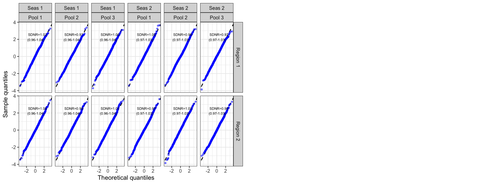

Population-specific index OSA (index_source = + pop = TRUE):

catch_pop_osa  <- get_osa(model = model_pop, data = input_pop$data, index_source = "Catch", pop = TRUE)
srvidx_pop_osa <- get_osa(model = model_pop, data = input_pop$data, index_source = "SrvIdx", pop = TRUE)

resid_catch_pop  <- plot_resids(catch_pop_osa)
resid_srvidx_pop <- plot_resids(srvidx_pop_osa)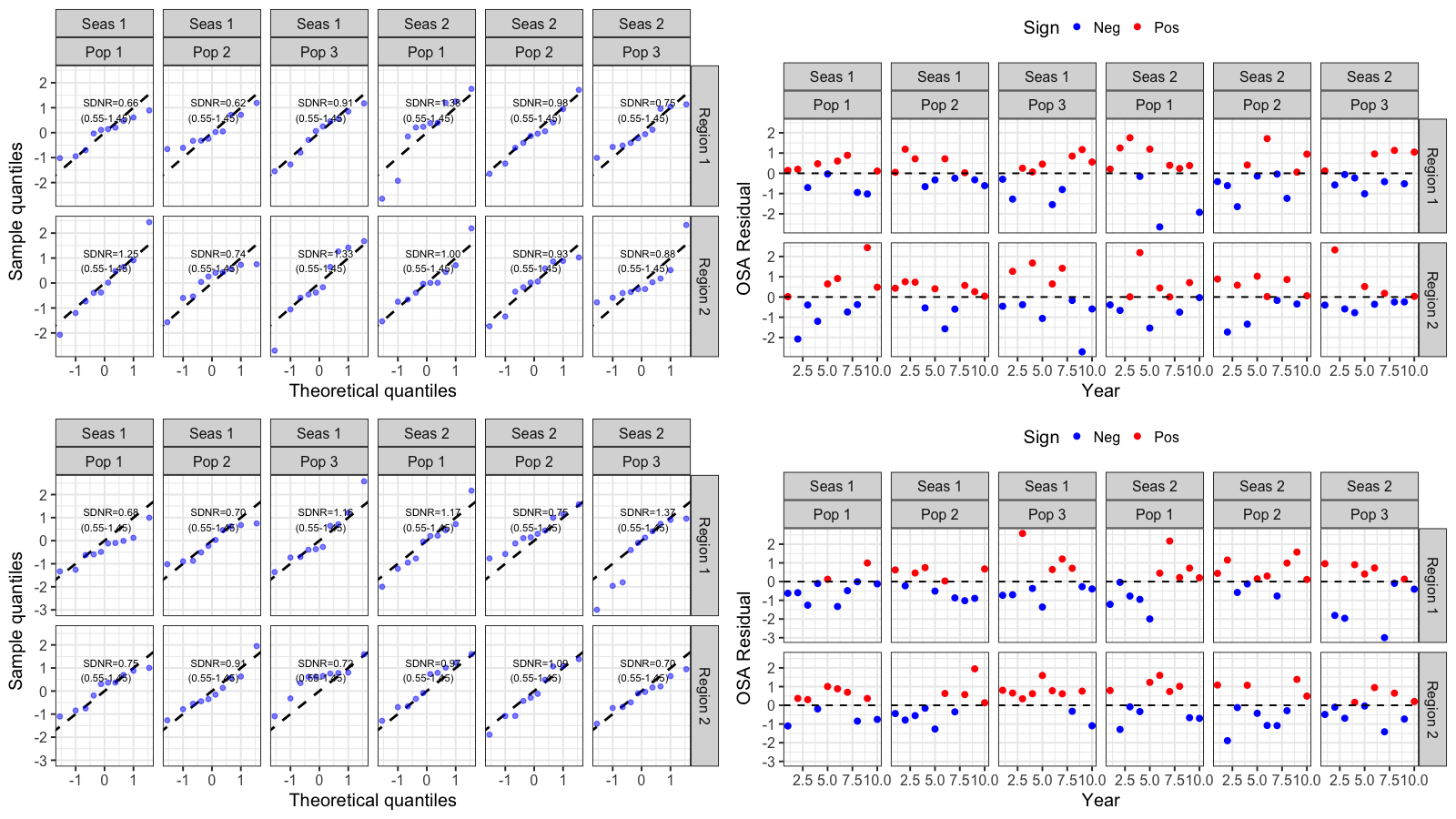

Covariates a dsem observes with error

A dsem whose covariates are observed with error fits those observations, so they have one-step-ahead residuals of their own, and dsem = TRUE returns them. A covariate left on dsem_family = "fixed" has no residual (since fixed) and hence doesn’t return anything here. We provide a contrived example below of how to call osa residuals below.

env <- data.frame(year = input_list$data$years, env = env_index)

input_dsem <- Setup_Mod_DSEM(
  input_list,
  dsem_arrows = c("env -> rec, 0, b_env", "env <-> env, 0, sd_env", "rec <-> rec, 0, sd_rec"),
  dsem_data = env,
  dsem_family = c(env = "normal")
)

model_dsem <- fit_model(input_dsem$data, input_dsem$par, input_dsem$map,
                        random = c("ln_RecDevs", "dsem_x"), newton_loops = 3, silent = TRUE)

dsem_osa <- get_osa(model = model_dsem, data = input_dsem$data, dsem = TRUE)
resid_dsem <- plot_resids(dsem_osa)

The residual data frame has a covariate column where the other sources have a fleet, and the plots facet on it when a dsem observes more than one. family picks between the covariates whose observations are continuous ("normal", "gaussian_fixed_sd", "gamma", "lognormal"), or one of "bernoulli", "poisson" and "tweedie", and defaults to the continuous ones. Those last three are asked for one at a time because each needs different arguments out of RTMB::oneStepPredict(), and those arguments hold for every observation in the call they are given: a bernoulli’s outcomes are 0 and 1, a poisson’s counts run past the largest one observed, and a tweedie’s zeros are named as a point mass with a range for the positive part. Each covariate keeps the density it was fit with, so a lognormal one gives the residual for the observation rather than for its log.

Other options

get_osa()’s internal mode uses three further arguments:

osa_method: overrides RTMB::oneStepPredict()’s method argument. Must be one of "oneStepGeneric", "oneStepGaussianOffMode", or "oneStepGaussian", the "cdf" method is deliberately disallowed because it is numerically unstable sometimes for the discrete (multinomial/count) likelihoods . Defaults to "oneStepGeneric" for discrete composition/tag families and "oneStepGaussianOffMode" for continuous (logistic-normal composition or index-type) families. A dsem’s covariates take "oneStepGeneric" whatever their family, and refuse a Gaussian method: a covariate’s state reaches its observation through the population model, so reading the conditional density’s curvature as its variance is wrong even for a normal covariate.
parallel: passed straight through to RTMB::oneStepPredict(parallel = ). Useful for large composition/tag datasets where OSA computation dominates runtime.
seed: the seed for the uniform draw that places a discrete residual inside its step of the CDF, which RTMB::oneStepPredict() fixes at 123 so that one call on one data set is reproducible.

get_osa(model = model, data = input_list$data, index_source = "SrvIdx",
       osa_method = "oneStepGaussian", parallel = TRUE)