Simulation Testing (Cross and Self Tests)
Source:vignettes/l_simulation_testing.Rmd
l_simulation_testing.RmdSimulation Cross-Testing in SPoRC
Simulation testing stock assessment models is integral to evaluating
robustness and understanding how models perform under model
misspecification. The SPoRC framework supports simulation
testing in three forms:
- Self-testing: the estimation model (EM) has the same structure as the
operating model (OM).
- Cross-testing: the EM differs structurally from the OM, allowing
assessment of bias and sensitivity to incorrect assumptions.
- Closed loop simulations (see Closed Loop Simulations vignette
example).
In this first section of the vignette, we present a cross-test
example. The operating model (OM; simulated truth) assumes a logistic
selectivity curve for the fishery, while the estimation model
(SPoRC; EM) incorrectly specifies a dome-shaped (gamma)
selectivity curve.
The OM defines the biological processes, fishing dynamics, survey structure, and recruitment assumptions. Unless otherwise noted, the OM observation model uses default settings:
- Composition Input Sample Size = 100, with Multinomial sampling (Fishery and Survey)
- Survey index SD = 0.2, with lognormal observations
- Catch SD = 0.02, with lognormal observations
Define Model Dimensions
We start by defining the structural dimensions of the operating model.
library(SPoRC)
library(dplyr)
library(ggplot2)

sim_list <- Setup_Sim_Dim(
  n_sims        = 50,  # number of simulations
  n_yrs         = 30,  # number of years
  n_regions     = 1,   # single region
  n_ages        = 10,  # number of ages
  n_lens        = NULL,# no length structure
  n_sexes       = 1,   # single sex
  n_fish_fleets = 1,   # one fishery fleet
  n_srv_fleets  = 1,    # one survey fleet
  n_pop         = 1    # number of pops
)

# Create storage containers
sim_list <- Setup_Sim_Containers(sim_list)
Fishing Processes
The fishery selectivity in the OM is logistic, centered around age 5.
sim_list <- Setup_Sim_Fishing(sim_list = sim_list, # update simulate list
                              # Logistic selectivity
                              fish_sel_input = replicate(
                                n = sim_list$n_sims,
                                array(rep(1 / (1 + exp(-3 * ((1:sim_list$n_ages) - 5))), each = sim_list$n_yrs),
                                      dim = c(sim_list$n_pop, sim_list$n_regions, sim_list$n_yrs, sim_list$n_seas, sim_list$n_ages,
                                              sim_list$n_sexes, sim_list$n_fish_fleets))
                              )
)
Survey Processes
We specify survey selectivity as logistic, centered around age 3.
sim_list <- Setup_Sim_Survey(
  sim_list = sim_list,
  # Logistic selectivity
  srv_sel_input = replicate(
    n = sim_list$n_sims,
    array(rep(1 / (1 + exp(-1 * ((1:sim_list$n_ages) - 3))), each = sim_list$n_yrs),
          dim = c(sim_list$n_pop, sim_list$n_regions, sim_list$n_yrs, sim_list$n_seas, sim_list$n_ages,
                  sim_list$n_sexes, sim_list$n_srv))
  )
)
Biological Dynamics
Biological parameters are set for natural mortality, maturity-at-age, and weight-at-age. These values are relatively arbitrary and are specified to generically represent a fairly short-lived species.
sim_list <- Setup_Sim_Biologicals(
  sim_list = sim_list, # simualtion list
  natmort_input = replicate(n = sim_list$n_sims, array(0.3, dim = c(sim_list$n_pop, sim_list$n_regions, sim_list$n_yrs,
                                                                    sim_list$n_ages, sim_list$n_sexes))), # natural mortality
  WAA_input = replicate(n = sim_list$n_sims, array(rep(5 / (1 + exp(-3 * ((1:sim_list$n_ages) - 3))), each = sim_list$n_yrs),
                                                   dim = c(sim_list$n_pop, sim_list$n_regions, sim_list$n_yrs, sim_list$n_seas, sim_list$n_ages, sim_list$n_sexes))), # weight at age
  WAA_fish_input = replicate(n = sim_list$n_sims, array(rep(5 / (1 + exp(-3 * ((1:sim_list$n_ages) - 3))), each = sim_list$n_yrs),
                                                        dim = c(sim_list$n_pop, sim_list$n_regions, sim_list$n_yrs, sim_list$n_seas, sim_list$n_ages, sim_list$n_sexes, sim_list$n_fish_fleets))), # fishery weight at age
  WAA_srv_input = replicate(n = sim_list$n_sims, array(rep(5 / (1 + exp(-3 * ((1:sim_list$n_ages) - 3))), each = sim_list$n_yrs),
                                                       dim = c(sim_list$n_pop, sim_list$n_regions, sim_list$n_yrs, sim_list$n_seas, sim_list$n_ages, sim_list$n_sexes, sim_list$n_srv_fleets))), # survey weight at age
  MatAA_input = replicate(n = sim_list$n_sims, array(rep(1 / (1 + exp(-3 * ((1:sim_list$n_ages) - 3))), each = sim_list$n_yrs),
                                                     dim = c(sim_list$n_pop, sim_list$n_regions, sim_list$n_yrs, sim_list$n_seas, sim_list$n_ages, sim_list$n_sexes))) # maturity at age
)
Tagging and Movement
For this example, tagging is disabled and no movement is modeled.
sim_list <- Setup_Sim_Tagging(
  sim_list = sim_list, # simulation list
  use_conv_fish_tagging = 0
)

# No Movement
sim_list$Movement <- array(1, dim = c(sim_list$n_pop, sim_list$n_regions, sim_list$n_regions, sim_list$n_yrs, sim_list$n_seas, sim_list$n_ages, sim_list$n_sexes, sim_list$n_sims))
Recruitment
Recruitment is modeled with mean recruitment dynamics, where
R0_input is the mean recruitment parameter centered at a
value of 5.
sim_list <- Setup_Sim_Rec(
  sim_list = sim_list,
  R0_input = replicate(n = sim_list$n_sims, expr = array(5, dim = c(sim_list$n_pop, sim_list$n_regions, sim_list$n_yrs))), # R0
  ln_sigmaR = array(log(1), dim = c(2, sim_list$n_pop, sim_list$n_regions)),
  recruitment_opt = 'mean_rec',
  init_age_strc = 1 # using geometric series scalar to initialize popn
)
Run the Operating Model
set.seed(123)
sim_obj <- Simulate_Pop_Static(sim_list = sim_list, output_path = NULL) # get simulated datasets
The object sim_obj contains the simulated population,
fishery, and survey data ready to pass to the EM for cross-testing.
Define Estimation Model
After simulating the operating model (OM), we can set up the
estimation model (EM) in SPoRC.
In this cross-test, the EM incorrectly assumes a dome-shaped (gamma)
fishery selectivity,
even though the OM used logistic selectivity. In general, EM settings
are identical to the OM, except for fishery selectivity.
setup_em <- function(sim_obj, sim) {

  # Extract simulation data for current year and replicate
  sim_data <- simulation_data_to_SPoRC(sim_env = sim_obj, y = sim_obj$n_years, sim = sim)

  # Setup model dimensions
  input_list <- Setup_Mod_Dim(
    years = 1:sim_obj$n_years,
    ages = 1:sim_obj$n_ages,
    lens = sim_obj$n_lens,
    n_regions = sim_obj$n_regions,
    n_sexes = sim_obj$n_sexes,
    n_fish_fleets = sim_obj$n_fish_fleets,
    n_srv_fleets = sim_obj$n_srv_fleets,
    n_pop = sim_obj$n_pop,
    verbose = FALSE
  )

  # Recruitment setup
  input_list <- Setup_Mod_Rec(
    input_list = input_list,
    do_rec_bias_ramp = 0, # not doing bias ramp
    sigmaR_switch = 1, # when to switch from early to late sigmaR (switch in first year)
    ln_sigmaR = array(log(1), dim = c(2, input_list$data$n_pop, input_list$data$n_regions)), # 2 values for early and late sigma
    rec_model = "mean_rec",
    sigmaR_spec = "fix", # fix early sigmaR and late sigmaR
    init_age_strc = 1, # geometric series to derive initial age structure
    equil_init_age_strc = 2, # estimating all intial age deviations
    ln_global_R0 = log(5)
  )

  # Biological setup
  input_list <- Setup_Mod_Biologicals(
    input_list = input_list,
    # Data inputs
    WAA = sim_data$WAA,
    MatAA = sim_data$MatAA,
    WAA_fish = sim_data$WAA_fish,
    WAA_srv = sim_data$WAA_srv,
    fit_lengths = 0, # not fitting lengths
    AgeingError = sim_data$AgeingError,
    M_spec = "fix",     # fixing natural mortality
    Fixed_natmort = array(0.3, dim = c(input_list$data$n_pop, input_list$data$n_regions, length(input_list$data$years),  length(input_list$data$ages), input_list$data$n_sexes))
  )

  # Movement and tagging
  input_list <- Setup_Mod_Tagging(input_list = input_list, use_conv_fish_tagging = 0)
  input_list <- Setup_Mod_Movement(
    input_list = input_list,
    use_fixed_movement = 1,
    Fixed_Movement = NA,
    do_recruits_move = 0
  )

  # Fishery catch & fishing mortality
  input_list <- Setup_Mod_Catch_and_F(
    input_list = input_list,
    # Data inputs
    ObsCatch = sim_data$ObsCatch,
    UseCatch = sim_data$UseCatch,
    # Model options
    Use_F_pen = 1,
    sigmaC_spec = "fix",
    # Fixing sigma C and F
    ln_sigmaC = sim_data$ln_sigmaC,
    ln_sigmaF = array(log(1), dim = c(input_list$data$n_regions, input_list$data$n_seas, input_list$data$n_fish_fleets))
    )

  # Survey selectivity and catchability
  input_list <- Setup_Mod_FishIdx_and_Comps(
    input_list = input_list,
    # Data inputs
    ObsFishIdx = sim_data$ObsFishIdx,
    ObsFishIdx_SE = sim_data$ObsFishIdx_SE,
    UseFishIdx = sim_data$UseFishIdx,
    ObsFishAgeComps = sim_data$ObsFishAgeComps,
    ObsFishLenComps = sim_data$ObsFishLenComps,
    UseFishAgeComps = sim_data$UseFishAgeComps,
    UseFishLenComps = sim_data$UseFishLenComps,
    ISS_FishAgeComps = sim_data$ISS_FishAgeComps,
    ISS_FishLenComps = sim_data$ISS_FishLenComps,
    # Model options
    fish_idx_type = c("biom"),
    FishAgeComps_LikeType = c("Multinomial"),
    FishLenComps_LikeType = c("none"),
    FishAgeComps_Type = c("agg_Year_1-terminal_Fleet_1"),
    FishLenComps_Type = c("none_Year_1-terminal_Fleet_1")
  )

  # Survey indices and compositions
  input_list <- Setup_Mod_SrvIdx_and_Comps(
    input_list = input_list,
    # Data inputs
    ObsSrvIdx = sim_data$ObsSrvIdx,
    ObsSrvIdx_SE = sim_data$ObsSrvIdx_SE,
    UseSrvIdx = sim_data$UseSrvIdx,
    ObsSrvAgeComps = sim_data$ObsSrvAgeComps,
    ObsSrvLenComps = sim_data$ObsSrvLenComps,
    UseSrvAgeComps = sim_data$UseSrvAgeComps,
    UseSrvLenComps = sim_data$UseSrvLenComps,
    ISS_SrvAgeComps = sim_data$ISS_SrvAgeComps,
    ISS_SrvLenComps = sim_data$ISS_SrvLenComps,
    # Model options
    srv_idx_type = c("biom"),
    SrvAgeComps_LikeType = c("Multinomial"),
    SrvLenComps_LikeType = c("none"),
    SrvAgeComps_Type = c("agg_Year_1-terminal_Fleet_1"),
    SrvLenComps_Type = c("none_Year_1-terminal_Fleet_1")
  )


  # Fishery selectivity and catchability
  input_list <- Setup_Mod_Fishsel_and_Q(
    input_list = input_list,
    # Model options
    fish_sel_model = c("gamma_Fleet_1"), # fishery selex model (NOTE: ASSUMES DOMED)
    fish_fixed_sel_pars_spec = c("est_all"), # whether to estiamte all fixed effects for fishery selectivity
    fish_q_spec = "est_all" # estimate fishery q
  )

  # Survey selectivity and catchability
  input_list <- Setup_Mod_Srvsel_and_Q(
    input_list = input_list,
    # Model options
    srv_sel_model = c("logist2_Fleet_1"), # survey selectivity form
    srv_fixed_sel_pars_spec = c("est_all"), # whether to estimate all fixed effects for survey selectivity
    srv_q_spec = c("est_all")  # whether to estiamte all fixed effects for survey catchability
  )

  # Data weighting
  input_list <- Setup_Mod_Weighting(
    input_list = input_list,
    Wt_Catch = 1,
    Wt_FishIdx = 1,
    Wt_SrvIdx = 1,
    Wt_Rec = 1,
    Wt_F = 1,
    Wt_Tagging = 0,
    Wt_FishAgeComps = array(1, dim = c(input_list$data$n_regions, length(input_list$data$years), input_list$data$n_seas,
                                       input_list$data$n_sexes, input_list$data$n_fish_fleets)),
    Wt_FishLenComps = array(1, dim = c(input_list$data$n_regions, length(input_list$data$years), input_list$data$n_seas,
                                       input_list$data$n_sexes, input_list$data$n_fish_fleets)),
    Wt_SrvAgeComps = array(1, dim = c(input_list$data$n_regions,length(input_list$data$years), input_list$data$n_seas,
                                      input_list$data$n_sexes, input_list$data$n_srv_fleets)),
    Wt_SrvLenComps = array(0, dim = c(input_list$data$n_regions, length(input_list$data$years), input_list$data$n_seas,
                                      input_list$data$n_sexes, input_list$data$n_srv_fleets))
  )

  return(input_list)

}
Run Cross-Test Analysis
After setting up the EM, we can run the cross-test by fitting the
model to each simulated dataset.
We store the resulting spawning stock biomass (SSB) estimates for
comparison with the OM.
ssb_results <- array(NA, dim = c(sim_list$n_yrs, sim_list$n_sims)) # storage container
for(i in 1:sim_obj$n_sims) {

  input_list <- setup_em(sim_obj, sim = i) # setup EM

  # fit model
  model <- fit_model(input_list$data,
                     input_list$par,
                     input_list$map,
                     random = NULL,
                     silent = TRUE
                     )

  ssb_results[,i] <- as.vector(model$rep$SSB) # save results

} # end i loop
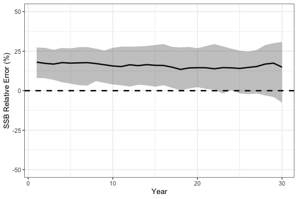
As expected, the simulation cross-test demonstrates that misspecification of fishery selectivity leads to biased estimates of key population quantities. In particular, spawning stock biomass (SSB) is positively biased because the EM incorrectly assumes dome-shaped selectivity while the true OM selectivity is logistic, treating a portion of the population as invulnerable to the fishery, leading to an overestimation of stock size.
# Process SSB results
ssb_df_res <- reshape2::melt(ssb_results) %>%
  rename(Year = Var1, Sim = Var2, Est = value) %>%
  dplyr::left_join(reshape2::melt(sim_obj$SSB) %>%
                     dplyr::rename(Region = Var2, Year = Var3, Sim = Var4, True = value), by = c("Year", "Sim")) %>%
  dplyr::mutate(RE = (Est - True) / True * 100) %>%
  dplyr::group_by(Year) %>%
  dplyr::summarize(median = median(RE, na.rm = TRUE),
                   lwr = quantile(RE, 0.1, na.rm = TRUE),
                   upr = quantile(RE, 0.8, na.rm = TRUE))

# plot!
print(
  ggplot(ssb_df_res, aes(x = Year, y = median, ymin = lwr, ymax = upr)) +
    geom_line(lwd = 1.3) +
    geom_hline(yintercept = 0, lwd = 1.3, lty = 2) +
    coord_cartesian(ylim = c(-50, 50)) +
    geom_ribbon(alpha = 0.3) +
    theme_bw(base_size = 15) +
    labs(x = 'Year', y = 'SSB Relative Error (%)')
)
Self Testing
In addition to simulation cross-testing, users can also conduct
self-tests. Simulation self-testing is useful because it helps evaluate
model robustness in the context of parameter identifiability. Ideally, a
simulation self-test should return unbiased parameter estimates on
average. If it does not, this generally indicates a lack of
identifiability for some parameters given the available data. Here, we
demonstrate simulation self-testing using Dusky Rockfish as an example.
Simulation self-testing is facilitated by the helper function
simulation_self_test, which allows users to conduct
simulations using a fitted SPoRC model (i.e., providing
data, parameters, mapping,
rep, and sd_rep). To reduce computation time,
we parallelize the simulations across 8 cores and output estimates of
SSB and recruitment.
# load in dusky rockfish model
data("dusky_rtmb_model")

# Using Dusky Rockfish as example to conduct simulation self-testing
self_test <- simulation_self_test(
  data = dusky_rtmb_model$data,
  parameters = dusky_rtmb_model$parameters,
  mapping = dusky_rtmb_model$mapping,
  random = NULL,
  rep = dusky_rtmb_model$rep,
  sd_rep = dusky_rtmb_model$sdrep,
  n_sims = 300,
  newton_loops = 3,
  do_sdrep = FALSE,
  do_par = TRUE,
  n_cores = 8,
  output_path = NULL,
  what = c("SSB", "Rec")
)
simulation_self_test has two designs. Under
sim_type = "conditional" (the default) every replicate runs
at the fitted parameters and the fitted process deviations, and only the
observations are drawn again, so the self test asks how well the data
return the population the fit describes. In theory the process sds come
back low under it, since the replicates run on deviations the fit has
already shrunk toward zero. Under sim_type = "joint" each
replicate draws its parameters from the fit’s joint precision
(RTMB::sdreport(obj, getJointPrecision = TRUE), passed with
obj), then every process from the penalty the estimation
model puts on it, then the observations, and is compared with its own
truth, so the self test asks whether the model recovers a population it
could itself have generated, process sds included. F deviations
estimated as penalized fixed effects are not redrawn: they come from the
parameter draw, and are drawn from their penalty only when the fit
integrates them out.
A fit with movement random effects (move_*_re in
Setup_Mod_Movement()) needs no additional setup. A
conditional self test and a closed loop’s fitted years keep the fit’s
deviations; a joint self test, and a closed loop’s projection years,
draw them from the process the estimation model penalizes and rebuild
the movement matrix before the population is run. An operating model
built by hand takes the same step through
Setup_Sim_Movement(), or Setup_Sim_DSEM() when
a dsem holds the deviations.
# a fit with AR1 movement deviations over years, sex-specific and correlated across sexes
input_list <- Setup_Mod_Movement(input_list, use_fixed_movement = 0, Fixed_Movement = NA,
                                 move_year_re = "ar1", move_sex_re = "us")
fit <- fit_model(input_list$data, input_list$par, input_list$map, random = "move_devs")

# an operating model built by hand: the fit's movement, then its deviation process
sim_list$Movement <- replicate(sim_list$n_sims, fit$rep$Movement)
sim_list <- Setup_Sim_Movement(sim_list, fit$data, fit$env$parList())
sim_env <- Setup_sim_env(sim_list) # every replicate now holds its own move_devs and Movement
A fit with growth deviations (growth_tv_model or
growth_semipar in Setup_Mod_Biologicals()) is
treated the same way, under the form the penalty gives them and the
fit’s maps, with weight at age, the size-age keys and selectivity at age
rebuilt through the fit’s own Get_Growth(); under cohort
growth the annual cycle advances growth from each replicate’s own
numbers at age. By hand the step is Setup_Sim_Growth_RE(),
which needs the fit’s report under selectivity at length.
# a fit with iid deviations on L1 and a random walk on K, their sds estimated
input_list <- Setup_Mod_Biologicals(input_list, ..., growth_tv_model = c(L1 = "iid", K = "rw"), growth_tv_sigma_spec = "est")
fit <- fit_model(input_list$data, input_list$par, input_list$map, random = "ln_growth_devs")

# an operating model built by hand: the fit's growth, then its deviation process
sim_list$WAA <- replicate(sim_list$n_sims, fit$rep$WAA) # and WAA_fish, WAA_srv, SizeAgeTrans_fish, SizeAgeTrans_srv the same way
sim_list <- Setup_Sim_Growth_RE(sim_list, fit$data, fit$env$parList(), rep = fit$rep)
sim_env <- Setup_sim_env(sim_list) # every replicate now holds its own ln_growth_devs and weight at age
Recruitment is treated the same way. A conditional self test runs
each replicate on the fit’s recruitment; a joint self test draws the
recruitment and initial age deviations from the penalties the fit puts
on them, under their form, bias ramp, sigma switch and weight, and a
deviation the fit leaves unpenalized or fixed keeps its value. An
operating model built by hand passes deviations of its own through
ln_RecDevs_input in Setup_Sim_Rec().
Priors and penalties need separate treatment. A prior’s mean is data
each refit reads but the self test does not redraw, so wherever the data
pulled the fit away from a prior every replicate is pulled back toward
it, a bias of the design rather than of the estimator.
prior_means = "truth" moves every prior onto the value the
replicate ran on and keeps its strength (the mean of a normal, the mode
of a Dirichlet or beta), "off" turns them off, and the
default "assessment" keeps them as given. A penalty that
describes a process is drawn from, as above; a penalty that regularizes,
such as the smoothing penalties on a bicubic selectivity surface, has
nothing to draw from, so any bias it shows is real. Recruitment
deviations estimated as penalized fixed effects rather than integrated
out tend to show a real bias too, an R0 that rises to reproduce the
indices from shrunk deviations, while spawning biomass, F and mean
recruitment stay close to the truth.
A fit with catchability deviations (fish_q_model or
srv_q_model) is treated the same way, each year the fit
estimates drawn under its form and each fixed year kept; by hand the
step is Setup_Sim_q_devs().
A fit with selectivity deviations (cont_tv_*_sel or the
bin-override deviations) is treated the same way, selectivity at age
rebuilt through the fit’s own Get_Selex_Array() and, at
length, read through each replicate’s own size-age key. F and discard
mortality deviations are drawn only when the fit integrates them out; as
fixed effects they come from the parameter draw, since their penalty is
a loose constraint rather than a description of how F varies
(F_devs_draw = "all" in Setup_Sim_Fleet_Devs()
draws them anyway). Three rules hold for every process: a penalty
weighted by Wt_* or *_pe_wt is drawn at its sd
over the square root of the weight and the refits keep the weight; a
random walk’s diffuse first year keeps the replicate’s own value, since
that start leaves the level to the data; and a cell the fit’s map fixes
keeps its value. A closed loop draws selectivity deviations on through
its projection years while F past the fit stays the control rule’s.
Simulate_Pop_Static() returns every draw.
The observations are drawn under the likelihood the fit evaluates
them with, so a self test refits data of the kind it was fit to: year
totals into the season the fit holds them in, an index with a partly
estimated sd at the sd the fit forms, a multivariate normal index over
its whole covariance, and pooled tag recaptures once per pool.
simulation_data_to_SPoRC() returns all of them.
A fit whose length compositions are recorded on coarser bins than the
population (LenBinMap in
Setup_Mod_Biologicals()), or are selected at length
(FishLenComps_sel or SrvLenComps_sel set to
"length"), also comes into the self test and the closed
loop without additional setup. The operating model maps each expected
length composition onto the recorded bins before drawing it, as the
estimation model maps it before evaluating the likelihood, and reads
each expected age composition and each age-at-length row through the
fleet’s ageing error the same way, so a simulated composition comes from
the distribution the fit evaluates. Under selectivity at length it
spreads the fish at each age over length and selects them length by
length from the fit’s selectivity at length, as the estimation model
does, and the conditional age-at-length is drawn from that same catch or
index at length and age. An operating model built by hand takes the map
through n_obs_lens in Setup_Sim_Dim() and
LenBinMap_input in Setup_Sim_Biologicals(),
and the selectivity at length through fish_sel_l_input and
ret_sel_l_input in Setup_Sim_Fishing() and
srv_sel_l_input in Setup_Sim_Survey().
Neither Setup_Sim_Movement() nor
Setup_Sim_Growth_RE() is required to read anything that an
optimizer produced; both only need data and a parameter
list in a fit’s own array shape, so a process error series can be
specified manually in place of an estimated one. This can be done with
the function Setup_Sim_Movement()’s own replicate loop
calls, matched to data and pars by
match_model_args() the same way; although both functions
are internal. Movement is self-contained enough that
Setup_Mod_Dim() and Setup_Mod_Movement() alone
give it everything it reads, with no input_list needed
beforehand either, the same way a pure cross-test never uses one:
# a bare input_list built from the OM's own dimensions, no EM or data involved
input_list <- Setup_Mod_Dim(years = 1:sim_list$n_yrs, ages = 1:sim_list$n_ages, lens = NULL,
                            n_regions = sim_list$n_regions, n_sexes = sim_list$n_sexes,
                            n_fish_fleets = sim_list$n_fish_fleets, n_srv_fleets = sim_list$n_srv_fleets,
                            n_pop = sim_list$n_pop)

# movement specified by hand instead of estimated
input_list <- Setup_Mod_Movement(input_list, use_fixed_movement = 0, Fixed_Movement = NA,
                                 move_year_re = "ar1", move_sex_re = "us")
input_list$par$move_pe_pars[] <- ... # chosen sd / correlation, not an estimate

move_args <- SPoRC:::match_model_args(SPoRC:::Get_Movement, input_list$data, input_list$par,
                                      n_yrs = sim_list$n_yrs, n_proj_yrs_devs = 0, n_ages = sim_list$n_ages)
movement <- do.call(SPoRC:::Get_Movement, move_args)

sim_list$Movement <- replicate(sim_list$n_sims, movement$Movement)
sim_list <- Setup_Sim_Movement(sim_list, input_list$data, input_list$par)
sim_env <- Setup_sim_env(sim_list) # every replicate now holds its own move_devs and Movement
Growth setup needs a little bit more, since Get_Growth()
also reads t_fish, t_srv,
spawn_seas and t_spawn, the within-season
timing that Setup_Mod_FishIdx_and_Comps(),
Setup_Mod_SrvIdx_and_Comps() and
Setup_Mod_Rec() would otherwise supply from real fleet
data. Plain placeholders for that timing, written onto data
directly, serve just as well when nothing is actually being fit:
# growth specified by hand instead of estimated, same dimensions plus length bins
input_list <- Setup_Mod_Biologicals(input_list, ..., growth_tv_model = c(L1 = "iid", K = "rw"), growth_tv_sigma_spec = "est")
input_list$par$growth_pe_pars[] <- ... # chosen sd, not an estimate

# the timing Setup_Mod_FishIdx_and_Comps / Setup_Mod_SrvIdx_and_Comps / Setup_Mod_Rec would otherwise supply
input_list$data$t_fish <- array(0, dim = c(input_list$data$n_regions, input_list$data$n_seas, input_list$data$n_fish_fleets))
input_list$data$t_srv <- array(0, dim = c(input_list$data$n_regions, input_list$data$n_seas, input_list$data$n_srv_fleets))
input_list$data$spawn_seas <- 1
input_list$data$t_spawn <- 0

growth_args <- SPoRC:::match_model_args(SPoRC:::Get_Growth, input_list$data, input_list$par, n_yrs = sim_list$n_yrs)
growth <- do.call(SPoRC:::Get_Growth, growth_args)

sim_list$WAA <- replicate(sim_list$n_sims, growth$WAA) # and WAA_fish, WAA_srv, SizeAgeTrans_fish, SizeAgeTrans_srv the same way
sim_list <- Setup_Sim_Growth_RE(sim_list, input_list$data, input_list$par, rep = NULL)
sim_env <- Setup_sim_env(sim_list) # every replicate now holds its own ln_growth_devs and weight at age
When no process error is wanted at all, none of this internal stuff
is needed either: sim_list$Movement and growth’s
sim_list$WAA / WAA_fish / WAA_srv
/ SizeAgeTrans_fish / SizeAgeTrans_srv can be
filled in directly, the same way the cross-test example above sets a
flat sim_list$Movement by hand.
Setup_Sim_Movement() and Setup_Sim_Growth_RE()
exist only to draw and rebuild a deviation series around those arrays;
skip both, and the internal calls above, once the arrays themselves are
what is being specified.
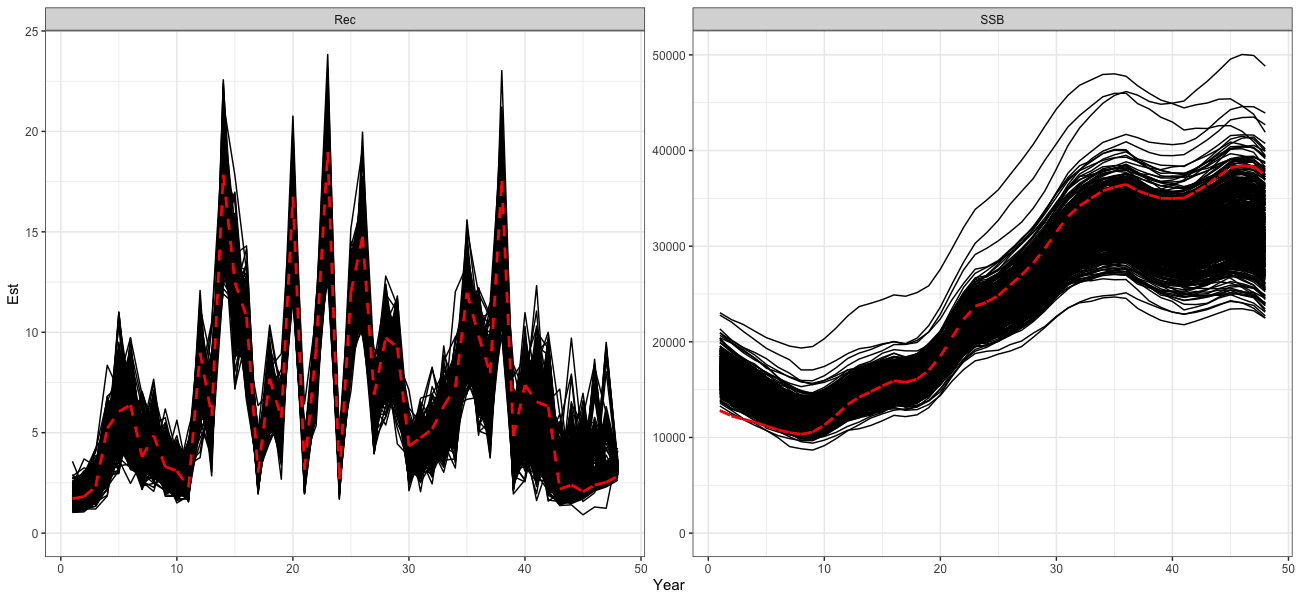
The self-test indicates that the model is generally able to recover the overall trends well. However, some biases manifest in the early and late periods, likely due to uncertainty in catch data in the early period and a lack of age composition data during these periods.
# Process self test results
self_test_res <- reshape2::melt(self_test$SSB) %>%
  dplyr::rename(Pop = Var1, Region = Var2, Year = Var3, Sim = Var4, Est = value) %>%
  dplyr::left_join(reshape2::melt(dusky_rtmb_model$rep$SSB) %>%
                     dplyr::rename(Region = Var2, Year = Var3, Best = value),
                   by = c("Region", "Year")) %>%
  dplyr::mutate(Type = 'SSB') %>%
  dplyr::bind_rows(
    reshape2::melt(self_test$Rec) %>%
  dplyr::rename(Pop = Var1, Region = Var2, Year = Var3, Sim = Var4, Est = value) %>%
      dplyr::left_join(reshape2::melt(dusky_rtmb_model$rep$Rec) %>%
                         dplyr::rename(Region = Var2, Year = Var3, Best = value),
                       by = c("Region", "Year")) %>%
      dplyr::mutate(Type = 'Rec')
  )

print(
  ggplot() +
    geom_line(self_test_res, mapping = aes(x = Year, y = Est, group = Sim)) +
    geom_line(self_test_res, mapping = aes(x = Year, y = Best), color = 'red', lty = 2, lwd = 1.3) +
    coord_cartesian(ylim = c(0, NA)) +
    facet_wrap(~Type, scales = 'free') +
    theme_bw(base_size = 15)
)