Choosing Growth Options

The size-age transition matrix is used in four places: length compositions are compared against it, length-based selectivity is applied through it, conditional age-at-length rows are read from it, and when weight at age is derived rather than supplied it converts numbers to biomass, and so enters spawning biomass and the reference points.

All of the options that build it are arguments to Setup_Mod_Biologicals(). This vignette covers what each one does and when to use it. The algebra is in vignette("c_model_equations") and the full argument list is in vignette("t_model_options"). Two case studies run the module end to end: vignette("ad_goa_rex_sole_case_study") for constant parametric growth with conditional age-at-length, and vignette("ae_ebs_pacific_cod_case_study") for time-varying growth kept cohort by cohort.

The examples use the packaged EBS Pacific cod inputs, which have length bins, a weight-length relationship and length compositions, so every option below can be switched on against them.

library(SPoRC)
data("sgl_rg_ebs_pcod_data")

dat <- sgl_rg_ebs_pcod_data
yrs <- dat$years; n_yrs <- length(yrs)
ages <- dat$ages; n_ages <- length(ages)
n_reg <- 1; n_sex <- 1

# lens are the bin midpoints the population is kept on; the transition is
# built on the lower edges, which is what growth_len_lower supplies
input_list <- Setup_Mod_Dim(
  years = yrs, ages = ages, lens = dat$lens,
  n_regions = n_reg, n_sexes = n_sex, n_fish_fleets = 1, n_srv_fleets = 1,
  n_seas = 1, n_pop = 1, natal_region = 1, verbose = FALSE
)

# Setup_Mod_Rec() has to run before the biologicals, because the maturity check
# reads rec_lag
input_list <- Setup_Mod_Rec(
  input_list = input_list, rec_model = "mean_rec", rec_lag = 0, t_spawn = 0,
  sigmaR_spec = "fix", ln_sigmaR = array(log(dat$rec$sigmaR), dim = c(2, 1, n_reg)),
  sigmaR_switch = 1, do_rec_bias_ramp = 0,
  init_age_strc = 2, equil_init_age_strc = 2, ln_global_R0 = dat$mle$ln_R0
)

Notation

Every symbol used below. Growth parameters additionally have population, region and sex subscripts $p, r, s$ , which are dropped throughout because sharing across them is a separate choice (growth_spec).

Symbol	Meaning	Kind
$a$	integer age class, $a = a_{1}, \dots, a_{+}$	index
$a_{+}$	accumulator age, holding every fish that old and older	index
$a^{\ast}$	first age past $A_{1}$ , where cohort propagation starts	index
$y$	model year	index
$\tau$	season, $\tau = 1, \dots, n_{\tau}$	index
$l$	length bin, $l = 1, \dots, n_{l}$	index
$d_{\tau}$	duration of season $\tau$ as a fraction of the year, $\sum_{\tau} d_{\tau} = 1$ (`seasdur`)	data
$t$	fraction of a season elapsed at a reading point (`t_fish`, `t_srv`, `t_spawn`)	data
$e$	fraction of the year elapsed at that reading point	derived
$x$	real age, $x = a + e$	derived
$\ell_{l}$	lower edge of length bin $l$ (`growth_len_lower`)	data
$\tilde{\ell}_{l}$	midpoint of length bin $l$ (`lens`)	data
$A_{1}, A_{2}$	reference ages for $L_{1}$ and $L_{2}$ (`growth_A1`, `growth_A2`)	data
$A_{2}^{cv}$	age at and above which $CV_{2}$ applies	data
$L_{0}$	length at age zero, anchoring the linear phase (`growth_L0`)	data
$L_{1}, L_{2}$	mean length at $A_{1}$ and at $A_{2}$	estimated
$K$	rate of approach to the asymptote	estimated
$\rho$	Richards coefficient; $\rho = 1$ under `"vb_schnute"`	estimated
$CV_{1}, CV_{2}$	spread parameters at the two reference ages	estimated
$L_{\infty}$	asymptotic length, solved from $L_{1}$ , $L_{2}$ , $K$	derived
$\bar{L}(x)$	mean length at real age $x$	derived
$\bar{L}_{+}$	mean length of the plus group	derived
$c(x)$	interpolated spread parameter at $x$	derived
$\sigma_{L}(x)$	standard deviation of length at $x$	derived
$g_{y}(L)$	growth increment over one year under year $y$ ’s parameters	derived
$A_{l,a}$	size-age transition, $P(\ell_{l} \mid a)$	derived
$N_{y,a}$	numbers at age at the start of year $y$	derived
$W_{a}$	weight at age	derived
$\delta_{y}$	time-varying deviation on a growth parameter in year $y$	estimated
$\varepsilon_{y,a}$	semi-parametric deviation on log mean length at age	estimated
$P, P^{lo}, P^{hi}$	a growth parameter and its bounds (`growth_par_bounds`)	see above
$\alpha, \beta$	weight-length parameters in $W = \alpha L^{\beta}$ (`wt_len_pars`)	data
$\Phi$	standard normal distribution function	function

Data or parameters

Under growth_model = "none", the default, SizeAgeTrans is data: an array [p x r x y x seas x l x a x s] of $P(\ell \mid a)$ built outside the model, column-stochastic, one slice per year and season. Weight at age is data too. Nothing about size is estimated.

Under growth_model = "vb_schnute" or "richards", the size-age transition is a function of five or six estimable parameters. SizeAgeTrans is then ignored and may be NA. One is built per fleet at that fleet’s timing (t_fish, t_srv), plus one at spawning time.

Use "none" if growth is determined externally and is not under study, if you are bridging an assessment that fixes it, or if there are no length data.

Use an estimated curve if you fit length compositions or conditional age-at-length, if size at age may have changed over the series, if growth uncertainty should propagate into the biomass, or if selectivity is length-based and would otherwise absorb a misspecified transition. The costs are parameters and tape-build time.

Prerequisites

The setup function will stop on each of these:

Requirement	Where
Length bin midpoints	`lens` in `Setup_Mod_Dim()`
`fit_lengths = 1`	`Setup_Mod_Biologicals()`
`growth_len_lower`	lower edges of those same bins, one per bin
`growth_A1`, `growth_A2`	the two reference ages the curve is anchored at

Which data you fit matters more than any switch below. Marginal length compositions identify the curve weakly, because a length distribution is a mixture over ages and abundance at age has to be separated from size at age. Conditional age-at-length constrains growth much more directly: a CAAL row is the age composition of the otoliths taken from one length bin, so it is informative about size at age and has little information about abundance. If you have aged otoliths with their lengths, fit them as CAAL (ObsSrv_caal, do_caal = 1) rather than as marginal age compositions.

The curve and its anchors

MatAA <- array(0, dim = c(1, n_reg, n_yrs, 1, n_ages, n_sex))
MatAA[1, 1, , 1, , 1] <- dat$MatAA

input_list <- Setup_Mod_Biologicals(
  input_list = input_list,
  WAA = NULL, MatAA = MatAA, AgeingError = dat$AgeingError,
  M_spec = "fix", Fixed_natmort = array(0.3866, dim = c(1, n_reg, n_yrs, n_ages, n_sex)),
  fit_lengths = 1, SizeAgeTrans = NA,
  growth_model = "vb_schnute",
  ln_growth_pars = array(log(c(L1 = 14, L2 = 100, K = 0.12, CV1 = 0.15, CV2 = 0.08)),
                         dim = c(1, n_reg, n_sex, 5)),
  growth_A1 = 1.5, growth_A2 = 20,
  growth_len_lower = dat$lens_lower, growth_L0 = dat$lens_lower[1],
  waa_model = "wt_len", wt_len_pars = dat$wtlen
)

WAA = NULL and SizeAgeTrans = NA because both come out of the growth module. The later sections change one argument of this call at a time; ... in them stands for the rest of it unchanged.

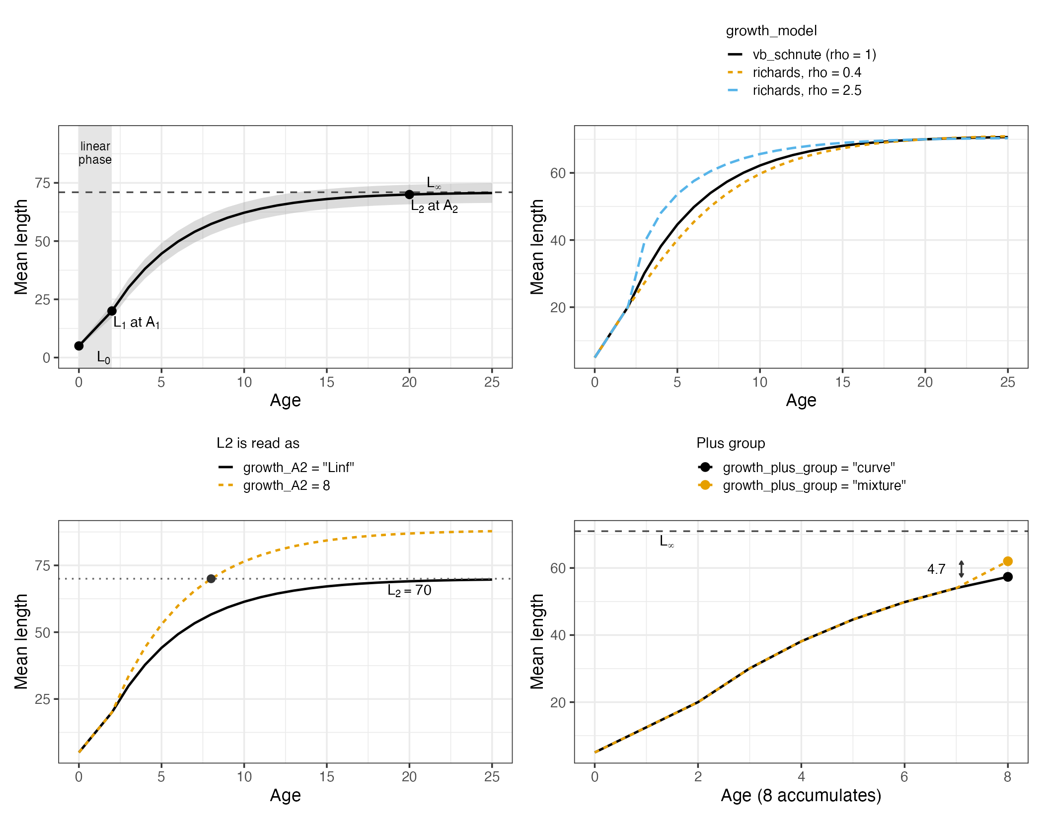
The Schnute curve and three of the switches that shape it. Top left: mean length at age, with the linear phase below growth_A1 shaded and a band one standard deviation either side of the mean. Top right: the Richards coefficient changes the shape of the approach to the asymptote, and equals von Bertalanffy at one. Bottom left: the same $L_{2}$ of 70 read as the length at age 8, from which the asymptote is solved, or read as the asymptote itself. Bottom right: the plus-group adjustment adds 4.7 cm at an accumulator age of 8.

Growth is parameterized in Schnute form rather than as $L_{\infty}$ , $K$ , $t_{0}$ . The parameters are lengths at named ages, so starting values can be read off a length-at-age scatter and bounds are lengths. Writing $x$ for real age (integer age plus the fraction of the year elapsed), and dropping the population, region and sex subscripts on every parameter:

$\bar{L}(x) = \begin{cases} L_{0} + \dfrac{x}{A_{1}}\left( L_{1} - L_{0} \right) & x < A_{1} \\[2ex] L_{\infty} + \left( L_{1} - L_{\infty} \right)e^{-K(x - A_{1})} & x \geq A_{1} \end{cases}$

with the asymptote solved from the two anchors,

$L_{\infty} = L_{1} + \frac{L_{2} - L_{1}}{1 - e^{-K(A_{2} - A_{1})}}$

and reported as Linf. The $L_{\infty}$ , $K$ , $t_{0}$ form is strongly correlated between $L_{\infty}$ and $K$ ; the Schnute form is less so, because each parameter is tied to an age with data behind it.

growth_model = "richards" applies the same curve to lengths raised to a power $\rho$ :

$\bar{L}(x)^{\rho} = L_{\infty}^{\rho} + \left( L_{1}^{\rho} - L_{\infty}^{\rho} \right)e^{-K(x - A_{1})}$

with $L_{\infty}^{\rho} = L_{1}^{\rho} + \left( L_{2}^{\rho} - L_{1}^{\rho} \right) / \left( 1 - e^{-K(A_{2} - A_{1})} \right)$ . At $\rho = 1$ this is the von Bertalanffy curve exactly, so the Richards form nests it. The linear phase below $A_{1}$ is unchanged.

growth_A1 and growth_A2 are data, not parameters. Set growth_A1 at or just above the youngest age in the length data, since below it the curve is a straight line from growth_L0 and is an assumption rather than a fit. Set growth_A2 old enough that fish are near the asymptote but young enough that the sample is not small.

growth_A2 = "Linf" reads $L_{2}$ as the asymptote itself, with no second reference age to solve it from. Use it when matching a source parameterized that way. The bottom-left panel shows that the same $L_{2}$ gives a different curve under each reading.

growth_L0 anchors the linear phase and defaults to the first length bin’s lower edge. It is rarely estimable, and only matters if recruits appear in the length compositions.

$\rho$ gives a more flexible approach to the asymptote at the cost of one parameter that is often unidentified. Start at $\rho = 1$ ; if the estimate barely moves and its standard error is large, use "vb_schnute".

The spread around the mean

The curve gives mean length at age. The size-age transition also needs a spread, set by three switches.

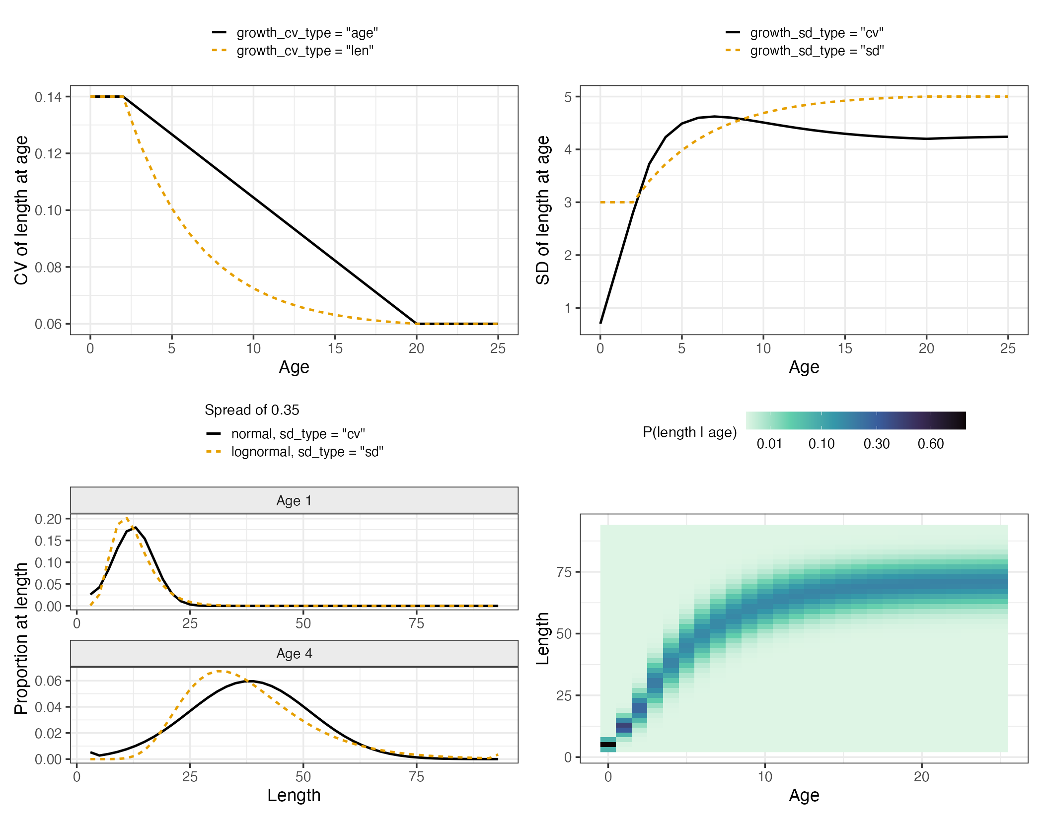
Top left: the CV runs from CV1 to CV2 between the reference ages, interpolated on mean length or on age. Top right: the same two parameters read as CVs, which scale the mean, or as standard deviations, which do not. Bottom left: the two dimensionally coherent pairings at a spread of 0.35, normal with growth_sd_type = "cv" and lognormal with "sd"; note the mass the normal puts in the smallest bin at age 1. Bottom right: the resulting size-age transition, on a square root color scale.

Two parameters hold the spread, $CV_{1}$ and $CV_{2}$ at the two reference ages, interpolated between them. growth_cv_type sets what the interpolation runs on:

$c(x) = \begin{cases} CV_{1} & x < A_{1} \\[1ex] CV_{1} + \left( CV_{2} - CV_{1} \right)\dfrac{\bar{L}(x) - L_{1}}{L_{2} - L_{1}} & A_{1} \leq x < A_{2}^{cv}, \quad \texttt{"len"} \\[2ex] CV_{1} + \left( CV_{2} - CV_{1} \right)\dfrac{x - A_{1}}{A_{2}^{cv} - A_{1}} & A_{1} \leq x < A_{2}^{cv}, \quad \texttt{"age"} \\[2ex] CV_{2} & x \geq A_{2}^{cv} \end{cases}$

where $A_{2}^{cv} = A_{2}$ , or the oldest age evaluated when growth_A2 = "Linf". The branch is taken on age either way; only the middle branch’s value depends on $\bar{L}(x)$ . The two agree at the reference ages and differ most where growth is fast, because interpolating on length compresses the change into the young ages. "len" is the Stock Synthesis convention; "age" gives a CV that declines steadily with age.

growth_sd_type then turns $c(x)$ into the standard deviation the transition is built from:

$\sigma_{L}(x) = \begin{cases} c(x)\,\bar{L}(x) & \texttt{"cv"} \\[1ex] c(x) & \texttt{"sd"} \end{cases}$

Under "cv" the spread scales with size, so a 20 cm and a 60 cm fish have standard deviations in the ratio 1:3. Under "sd" the absolute spread is the same at every age. "cv" gives an implausibly tight distribution at the youngest ages when the linear phase runs down to a very small growth_L0; use "sd" in that case. A CV that declines with size ( $CV_{2} < CV_{1}$ ) is the usual estimate, since the lengths of young fish vary with birth date and early growth while old fish have converged on the asymptote.

growth_dist sets the distribution that is binned. The two are close at the spreads most assessments estimate; the panel above uses 0.35 to make the difference visible. Use "lognormal" when the spread is large enough that a normal puts appreciable mass below zero length.

Note the pairing. The transition is always built from the $\sigma_{L}(x)$ that growth_sd_type produced, and the lognormal transform reads it as a log-scale standard deviation. So "lognormal" belongs with growth_sd_type = "sd"; combining it with "cv" passes a length-scale spread into a log-scale transform.

The plus group

The accumulator age holds every fish that old and older, so its mean size is not the curve’s value there.

growth_plus_group = "mixture", the default, treats it as a mixture of the ages it contains. The share of fish $k$ years past the accumulator age $a_{+}$ is taken as proportional to $e^{-0.2k}$ , the survivorship under a total mortality of 0.2 per year, and mean length is taken to rise linearly from $\bar{L}(a_{+})$ to $L_{\infty}$ over a second lifetime of $a_{+}$ years:

$\bar{L}_{+} = \frac{\sum_{k=0}^{a_{+}} e^{-0.2k}\left[ \bar{L}(a_{+}) + \dfrac{k}{a_{+}}\left( L_{\infty} - \bar{L}(a_{+}) \right) \right]}{\sum_{k=0}^{a_{+}} e^{-0.2k}}$

The 0.2 is a fixed assumption about how fast numbers decline with age, not an estimated rate, and it sets how much weight the older and larger fish have. $\bar{L}_{+}$ lies between $\bar{L}(a_{+})$ and $L_{\infty}$ . growth_plus_group = "curve" uses $\bar{L}(a_{+})$ directly.

The two agree closely when the accumulator age is old enough that little growth remains, and diverge as the plus group moves younger. With an accumulator age well short of the asymptote, "curve" undersizes the plus group and shifts its length composition left.

Binning

The mean and the spread are turned into the size-age transition by integrating the distribution over each length bin. With $\ell_{l}$ the lower edge of bin $l$ , each edge is standardized,

$z_{l,a} = \frac{\ell_{l} - \bar{L}(a)}{\sigma_{L}(a)}$

and each bin takes the probability between its edges, with the two tails accumulated into the end bins:

$A_{l,a} = \begin{cases} \Phi(z_{2,a}) & l = 1 \\[1ex] \Phi(z_{l+1,a}) - \Phi(z_{l,a}) & 1 < l < n_{l} \\[1ex] 1 - \Phi(z_{n_{l},a}) & l = n_{l} \end{cases}$

The column sums to one for any $\bar{L}(a)$ and $\sigma_{L}(a)$ , including means outside the binned range entirely, which is what makes each column a proper $P(\ell \mid a)$ . Under growth_dist = "lognormal" the same differences are taken on the log scale, about a median-corrected mean so that $E[L] = \bar{L}(a)$ :

$z_{l,a} = \frac{\log \ell_{l} - \left( \log \bar{L}(a) - \sigma_{L}^{2}(a)/2 \right)}{\sigma_{L}(a)}$

$\sigma_{L}(a)$ sets how many bins an age’s mass spreads over: large values flatten the column, small ones concentrate it near $\bar{L}(a)$ .

Timing within the year

Growth parameters are annual. growth_pars_y has no season dimension, and none of $L_{1}, L_{2}, K, CV_{1}, CV_{2}, \rho$ changes within a year. What changes within the year is the age the curve is evaluated at.

Where each reading point falls

Each fleet reads its own size-age transition and weight at age at the point its observations are taken: fishery fleet $f$ at $t^{fish}_{\tau,f}$ , survey $g$ at $t^{srv}_{\tau,g}$ , and the spawning weight at $t^{spawn}$ in the spawning season. Each $t$ is a fraction of its own season, in $[0, 1]$ , not a fraction of the year.

Converting one to a fraction of the year gives the elapsed time $e$ . For a reading at fraction $t$ of season $\tau$ :

$e(\tau, t) \;=\; \underbrace{\sum_{\tau' = 1}^{\tau - 1} d_{\tau'}}_{\text{seasons already completed}} \;+\; \underbrace{t\, d_{\tau}}_{\text{part of season } \tau \text{ elapsed}}$

where $d_{\tau'}$ is the duration of season $\tau'$ as a fraction of the year, from seasdur, and the seasons sum to a year, $\sum_{\tau = 1}^{n_{\tau}} d_{\tau} = 1$ . The empty sum is zero, so $e(1, 0) = 0$ is the start of the year.

The curve is then evaluated at the real age

$x_{a} = a + e(\tau, t)$

for every age class $a$ , giving $\bar{L}(x_{a})$ and $\sigma_{L}(x_{a})$ from the same two equations as before. Nothing is interpolated between integer ages.

A worked example, four equal quarters so $d_{\tau} = 0.25$ for all $\tau$ , with a survey read at the midpoint of the third quarter, $\tau = 3$ and $t = 0.5$ :

$e = (0.25 + 0.25) + 0.5 \times 0.25 = 0.625$

so an age 4 fish is placed at $x = 4.625$ on the curve. Note that $t = 0.5$ puts the reading halfway through that quarter, not halfway through the year. With a single season, $d_{1} = 1$ , the two coincide and $t = 0.5$ does give $x = a + 0.5$ .

Why seasons add no approximation

Write the one-year increment under year $y$ ’s parameters as

$g_{y}(L) = \left[ L_{\infty,y}^{\rho_{y}} + \left( L^{\rho_{y}} - L_{\infty,y}^{\rho_{y}} \right)e^{-K_{y}} \right]^{1/\rho_{y}}$

and the same map over an arbitrary elapsed time $e$ as $g_{y}(L; e)$ , which replaces $e^{-K_{y}}$ with $e^{-K_{y}e}$ . Applied to a length already on the curve it returns the curve’s own value $e$ later:

$g_{y}\!\left( \bar{L}(x);\, e \right) = \bar{L}(x + e)$

The identity is exact for the von Bertalanffy form and holds to machine precision for the Richards form (a maximum absolute difference of $3 \times 10^{-14}$ cm at $\rho = 0.4$ and $\rho = 2.5$ ). Because the module evaluates $\bar{L}(x_{a})$ directly rather than stepping season by season, the season structure cannot introduce error: with growth constant over years, the same mean length at age comes out whatever $n_{\tau}$ and $d_{\tau}$ are.

Only distinct values of $e$ within a season are evaluated, so fleets sharing a timing cost nothing extra.

The two exceptions

Two quantities are advanced by $g_{y}(\cdot\,; e)$ rather than read off the curve, because neither sits on it:

$\bar{L}_{\tau,a} = \begin{cases} g_{y}\!\left( \bar{L}_{+};\, e \right) & a = a_{+} \\[1.5ex] g_{y}\!\left( \bar{L}_{y,a};\, e \right) & a \geq a^{\ast}, \quad \texttt{growth\_tv\_type = "cohort"} \\[1.5ex] \bar{L}(x_{a}) & \text{otherwise} \end{cases}$

The plus group starts from its mixture-adjusted size $\bar{L}_{+}$ , which is a weighted average of ages rather than a point on the curve. Under cohort growth, every age at or past $a^{\ast}$ starts from $\bar{L}_{y,a}$ , the size that cohort actually reached.

# one curve per sex, shared across regions, with the second CV kept fixed
input_list <- Setup_Mod_Biologicals(
  input_list = input_list, ...,
  growth_model = "vb_schnute",
  growth_spec = "est_shared_r",
  growth_fix = c(L1 = FALSE, L2 = FALSE, K = FALSE, CV1 = FALSE, CV2 = TRUE)
)

growth_spec uses the same vocabulary as every other _spec argument: "est_all" (one set per population, region and sex), "est_shared_r", "est_shared_s", "est_shared_r_s", or "fix". growth_fix overrides it for individual parameters, holding named ones at their starting values regardless of the sharing.

Sex: if the sexes differ in size at age and the compositions are sex-split, estimate them separately. Sharing growth across sexes that differ leaves the difference to be absorbed by selectivity.

Region: share across regions unless there are regional length data to identify a difference.

CV2 is usually the first parameter to fix, since it is informed only by the oldest ages, where samples are small and the plus group confounds it. Fix rho at one unless it moves.

Starting values matter here more than in most parts of the model. ln_growth_pars defaults to the ends of the length bins with a rate of 0.15 and CVs of 0.1, which is a placeholder rather than a prior. Supply your own on the log scale, dimensioned [n_pop x n_regions x n_sexes x n_gpars] in the order L1, L2, K, CV1, CV2 and then rho. An external growth fit, even a rough one, is a reasonable starting point.

Growth that changes over time

There are two mechanisms, and they can be used together.

Varying the parameters

input_list <- Setup_Mod_Biologicals(
  input_list = input_list, ...,
  growth_model = "richards",
  growth_tv_model = c(L1 = "iid", K = "iid"),
  growth_tv_years = list(L1 = 2000:2024, K = 2000:2024),
  growth_tv_link = "logit",
  growth_par_bounds = dat$growth$bounds,
  growth_tv_sigma_spec = "fix",
  growth_tv_type = "cohort"
)

growth_tv_model names a structure per parameter, "none", "iid" or "rw", either as a vector in parameter order or named with the rest left constant. Each varying parameter gains a deviation series in ln_growth_devs and a process error standard deviation. Growth parameters trade off against each other, so letting all five vary at once tends to give a well-fitting series that is hard to interpret. Name only the parameters you have a reason to move.

growth_tv_years restricts each parameter’s deviations to given calendar years, as a vector applied to all of them or a list named per parameter. Deviations outside the range are kept at zero. Use the years in which the length data are informative.

growth_tv_link sets the scale the deviation enters on. For a base parameter $P$ with deviation $\delta_{y}$ , the value in year $y$ is

$P_{y} = \begin{cases} P\exp(\delta_{y}) & \texttt{"log"} \\[1ex] P^{lo} + \left( P^{hi} - P^{lo} \right)\,\mathrm{logit}^{-1}\left[ \mathrm{logit}\!\left( \dfrac{P - P^{lo}}{P^{hi} - P^{lo}} \right) + \delta_{y} \right] & \texttt{"logit"} \end{cases}$

The log link is unbounded and can drive a CV negative or a $K$ to an implausible value. The logit link keeps the parameter strictly inside $(P^{lo}, P^{hi})$ from growth_par_bounds however large the deviation. Growth parameters are all bounded by construction, so "logit" with sensible bounds is the better default. The realized $P_{y}$ are reported as growth_pars_y.

growth_tv_sigma_spec holds the process error standard deviations at their starting values ("fix") or estimates them ("est"). The starting values are the first data source of growth_pe_pars, one slot per growth parameter. Fixing them makes the deviations a penalized-likelihood problem in which you set how much variation is allowed. Estimating them requires the deviations to be integrated out; see below.

growth_tv_spec shares the deviation series across regions and sexes with the same vocabulary as growth_spec. A deviation series per stratum adds parameters quickly, so this is often worth sharing even when the base parameters are not. growth_rw_init_sigma gives the first year of a random walk its own standard deviation, defaulting to 5, which leaves the starting point close to free.

Curve or cohort

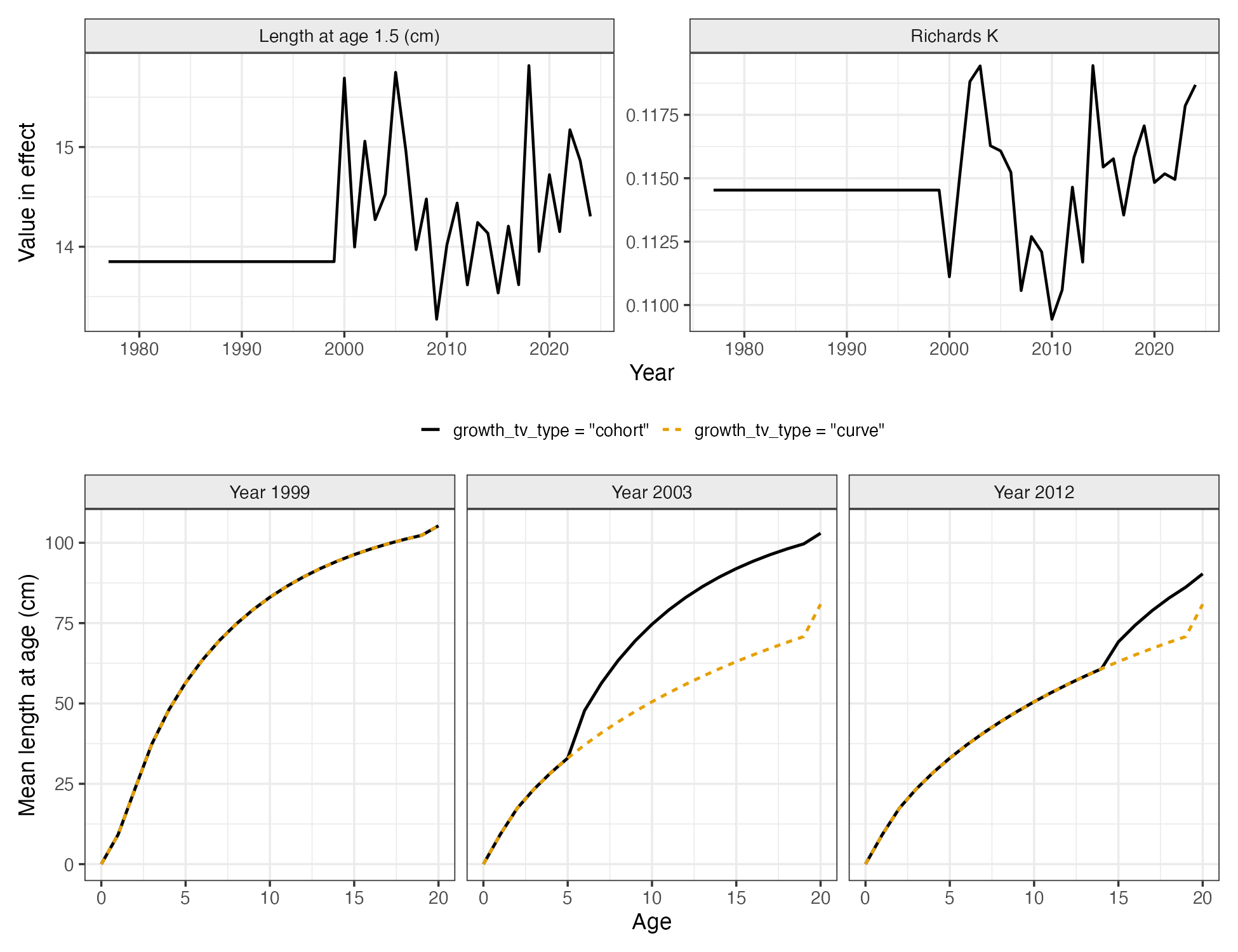
Top: the two growth parameters that vary in the EBS Pacific cod model, as the assessment’s estimate realizes them year by year. Bottom: what the same deviations do to mean length at age under each reading. The assessment’s deviations are small enough that the two nearly coincide, so the bottom panel exaggerates them into one sustained drop in $K$ from 2000 to make the mechanism visible. It is an illustration, not the assessment’s estimate.

growth_tv_type = "curve", the default, reads every year’s sizes off that year’s curve. Nothing is kept between years: if $K$ drops, every age is immediately shorter, including fish that grew through twenty prior years. Use it when the deviations represent something acting on all ages at once, or when the curve describes the population sampled in a year rather than a growth process.

"cohort" has size at age forward instead. Writing $g_{y}$ for the growth increment over one year under year $y$ ’s parameters,

$g_{y}(L) = \left[ L_{\infty,y}^{\rho_{y}} + \left( L^{\rho_{y}} - L_{\infty,y}^{\rho_{y}} \right)e^{-K_{y}} \right]^{1/\rho_{y}}$

the start-of-year mean length advances as

$\bar{L}_{y+1,a} = \begin{cases} L_{0} + \dfrac{a}{A_{1}}\left( L_{1,\,y+1-a} - L_{0} \right) & a < A_{1} \\[2ex] \bar{L}_{y+1}(a) & a = a^{\ast} \\[2ex] g_{y}\left( \bar{L}_{y,a-1} \right) & a^{\ast} < a < a_{+} \\[2ex] \dfrac{\left( N_{y,a_{+}-1} + 0.01 \right)g_{y}\left( \bar{L}_{y,a_{+}-1} \right) + \left( N_{y,a_{+}} + 0.01 \right)g_{y}\left( \bar{L}_{y,a_{+}} \right)}{N_{y,a_{+}-1} + N_{y,a_{+}} + 0.02} & a = a_{+} \end{cases}$

with $a^{\ast}$ the first age past $A_{1}$ . Three things follow. Ages still in the linear phase take the length at $A_{1}$ their birth year’s parameters gave them, so a cohort born in a poor year has that start forward. The plus group blends the cohort entering it with the fish already there by their numbers at age, which is the only place growth depends on abundance. And a poor growth year tracks the affected cohorts up through the ages for the rest of the series. Use it when the deviations represent conditions a fish lived through.

Two consequences of "cohort": because the plus group reads abundance, growth is evaluated inside the population dynamics year loop and the model costs more to tape; and $c(x)$ is evaluated once from the first year’s curve and then kept while the mean moves, so the deviations change mean size without also changing the spread.

Semi-parametric growth

growth_semipar adds a year-by-age surface of deviations multiplying the parametric mean length at age,

$\bar{L}_{y,a}^{\ast} = \bar{L}_{y,a}\exp\left( \varepsilon_{y,a} \right)$

applied after the curve and after any cohort propagation. The curve remains the parametric part and $\varepsilon$ holds departures from it. This represents changes in the shape of size at age that no parameter of the curve can express: a curve with five parameters cannot fit a year in which only the four-year-olds were small, and an unconstrained transition per year is not identified.

input_list <- Setup_Mod_Biologicals(
  input_list = input_list, ...,
  growth_model = "vb_schnute",
  growth_semipar = "2dar1",
  growth_semipar_spec = "est",
  growth_semipar_ages = 2:12,
  growth_semipar_years = 1990:2024
)

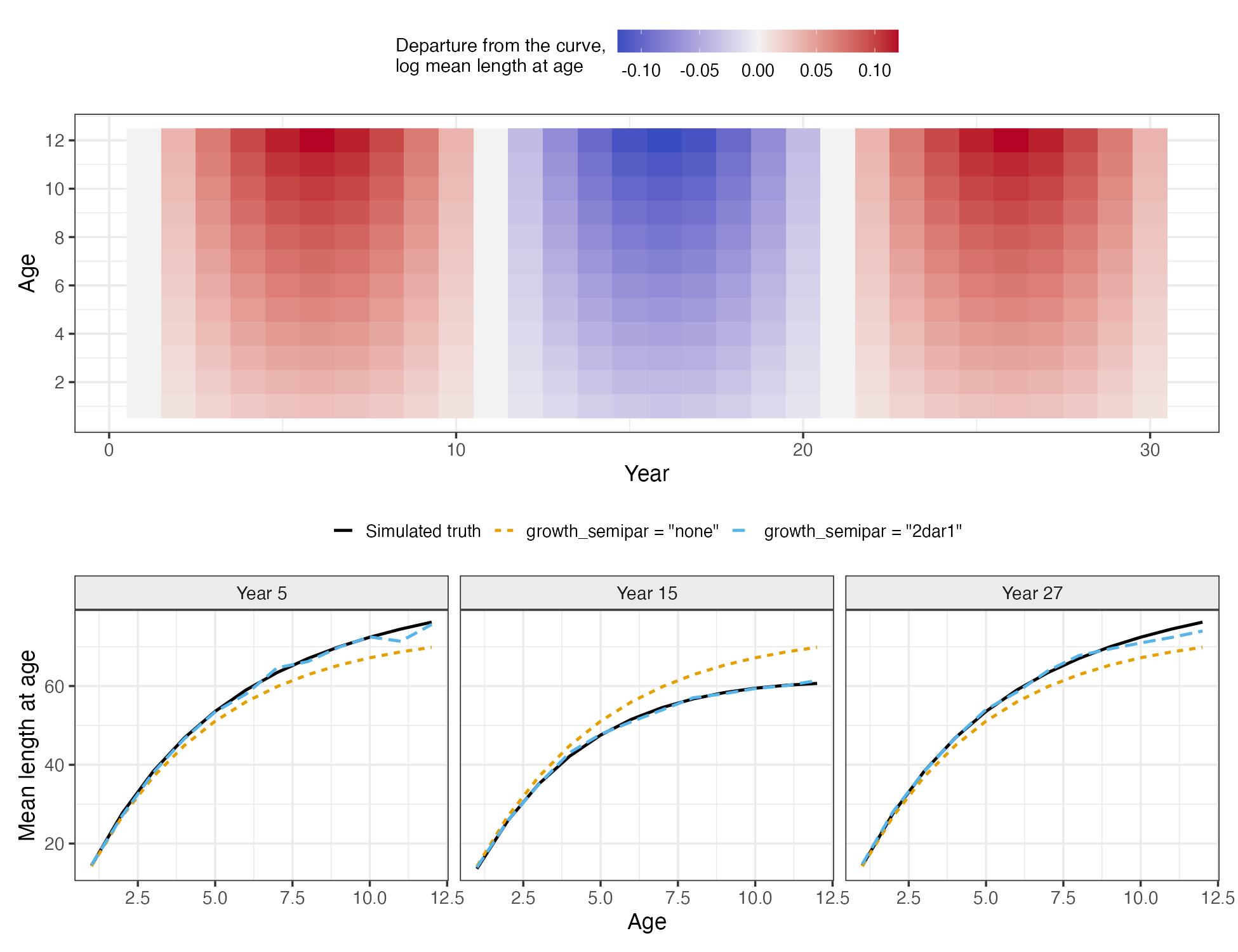
Top: a known year-by-age surface used to simulate length compositions and conditional age-at-length. Bottom: mean length at age recovered from those data by a model with a 2D AR(1) surface and by one with the parametric curve alone, against the truth. Over the whole surface the semi-parametric model is within 8.9% of the simulated mean length at age; the parametric curve alone is within 15.8%.

The available forms are the process errors semi-parametric selectivity uses: "iid", "rw" (a random walk over years within an age), "2dar1" (a separable first-order autoregression over ages and years), and "3dmarg" / "3dcond" (a three-dimensional Gaussian Markov random field over age, year and cohort, on the marginal or conditional variance).

The correlated forms are what make the surface estimable. A year-by-age deviation is not identified from length data one cell at a time, so the process error has to borrow strength across neighboring cells. "iid" provides none of that and is mainly useful as a null. "2dar1" is a reasonable default. The 3D forms add a hyperparameter and correlate along the cohort diagonal as well as over ages and years, which is worth it when a cohort signal is expected.

growth_semipar_ages and growth_semipar_years hold deviations outside them at zero. Restrict the surface to the ages and years the length data cover; elsewhere it adds unconstrained parameters.

The spread follows the deviated mean, so under growth_cv_type = "len" a deviation that lengthens a fish also moves it along the CV ramp. Under "age" the spread at age is unaffected.

The surface and the parametric time variation compose. Use the parameters for changes that can be attributed to a named mechanism and the surface for the residual, and avoid asking both to explain the same variation.

Why the two deviation data sources are separate

They are indexed over different dimensions and applied at different points:

ln_growth_devs         # [n_pop, n_regions, n_yrs, n_gpars, n_sexes]  4th dim: parameter
ln_growth_semipar_devs # [n_pop, n_regions, n_yrs, n_ages,  n_sexes]  4th dim: age

ln_growth_devs is applied before the curve is evaluated, perturbing L1, L2, K, CV1, CV2 and rho. ln_growth_semipar_devs multiplies mean length at age after the curve and after any cohort propagation.

Three things follow from that. The correlated process errors correlate over age, year and cohort, which is only meaningful when the index is age, so "2dar1" and the 3D forms are available to the surface and not to the parametric data source, where "iid" and "rw" are the only sensible structures. Cohort propagation works off the growth increment the year’s parameters imply, so it acts on the parametric data source; the surface multiplies in afterwards and is not kept forward. And parametric deviations keep size at age inside the curve’s shape, whereas the surface lets it leave.

The two data sources do share one array, growth_pe_pars: slot [,,,,1] holds the time-varying standard deviations and [,,,,2] the surface’s hyperparameters, with slots a given form does not read mapped off.

Deviations as random effects

Both data sources can be integrated out with the Laplace approximation instead of penalized, as selectivity deviations are in vignette("n_single_region_ebs_pollock_randomeff_case_study"). Pass the parameter name to fit_model():

# time-varying growth parameters, with their process error estimated
fit <- fit_model(input_list$data, input_list$par, input_list$map,
                 random = "ln_growth_devs", newton_loops = 3, silent = TRUE)

# a semi-parametric surface, or both together
fit <- fit_model(input_list$data, input_list$par, input_list$map,
                 random = c("ln_growth_devs", "ln_growth_semipar_devs"),
                 newton_loops = 3, silent = TRUE)

This is what growth_tv_sigma_spec = "est" and growth_semipar_spec = "est" require. Maximizing over a process error standard deviation and the deviations it penalizes at the same time, with both as fixed effects, drives the standard deviation toward zero. Integrating the deviations out makes it a variance parameter the data can inform. With the process error fixed, the fixed-effect treatment is fine and cheaper.

fit_model() uses the tape Hessian for its Newton refinement only when there are no random effects, so a random-effects fit takes the slower path.

Weight at age

input_list <- Setup_Mod_Biologicals(
  input_list = input_list,
  WAA = NULL, MatAA = MatAA, ...,
  growth_model = "richards",
  waa_model = "wt_len", wt_len_pars = dat$wtlen  # a, b in W = a L^b
)

waa_model = "data", the default, reads WAA, WAA_fish and WAA_srv from the arguments of the same name.

waa_model = "wt_len" builds them from the size-age transition and the weight-length relationship $W = \alpha L^{\beta}$ applied at the bin midpoints $\tilde{\ell}_{l}$ :

$W_{a} = \sum_{l} A_{l,a}\,\alpha\,\tilde{\ell}_{l}^{\beta}$

Weight at age then reflects the spread of length at age rather than being the weight of the mean length, which differ when $\beta \neq 1$ . The spawning weight uses the transition at spawning time and each fleet’s weight the transition at that fleet’s timing, so weight at age becomes fleet-specific, and time-varying whenever growth is. WAA may be NULL.

Use "wt_len" when growth is estimated and the biomass should inherit its uncertainty and time variation. Use "data" when empirical weight at age is available, which is generally better than a weight-length relationship, or when matching an assessment that supplies it.

Under "wt_len" the weight arrays are model output, but reference point and projection code read data$WAA. Copy the reported arrays into the data list before calling Get_Reference_Points() or Do_Population_Projection():

rep <- fit$rep
input_list$data$WAA <- rep$WAA
input_list$data$WAA_fish <- rep$WAA_fish
input_list$data$WAA_srv <- rep$WAA_srv

A related switch sits with the fleets rather than here: fish_waa_selected and srv_waa_selected put catch and index biomass on the selection-weighted weight at age, which applies only with length-based selectivity and a derived weight.

Compositions on coarser bins

LenBinMap maps the model’s length bins onto the bins the compositions are recorded on, a matrix [n_lens x n_obs_lens] whose rows sum to one. Growing fish on fine bins and fitting them on coarse ones gives a smoother transition and better-behaved tails while keeping the compositions on the bins they were collected on. The expected compositions are mapped through it inside the likelihood, as the ageing error matrix maps ages.

Checking the setup

Setup_Mod_Biologicals() prints what it built when verbose = TRUE. The EBS Pacific cod setup, with a semi-parametric surface added on top, reports:

Growth is estimated (Richards); SizeAgeTrans is built inside the model
Growth parameters varying over time: L1 (iid), K (iid); link logit; size at age
  read from cohort propagation from 2000
Weight at age (spawning, fishery, survey) is derived from growth and the
  weight-length relationship
Semi-parametric growth: 2dar1 deviations on mean length at age over 48 years
  and 11 ages, process error fix
Length compositions are recorded on 24 bins, mapped from the model's 121 bins
  inside the likelihood

That covers which parameters vary and how, the link, the year cohort propagation starts from, how many ages the surface covers, and where weight at age comes from.

After fitting, the report contains:

Field	What it holds
`growth_pars_y`	the parameters in effect, `[p x r x y x 6 x s]`
`Linf`	the derived asymptote, `[p x r x y x s]`
`L_beg`	mean length at age at the start of the year
`mean_LAA_fish`, `mean_LAA_srv`, `mean_LAA_spawn`	mean length at age at each fleet’s timing and at spawning
`sd_LAA_*`	the matching spreads
`SizeAgeTrans_fish`, `SizeAgeTrans_srv`, `SizeAgeTrans_spawn`	the size-age transitions
`growth_tv_nLL`, `growth_semipar_nLL`	the deviation penalties

Plot growth_pars_y against year before interpreting a time-varying fit, and mean_LAA_* in a few years against any external length-at-age data. A growth series that swings without an identifiable mechanism is usually absorbing something else, most often selectivity or a change in sampling.

Summary

Question	Argument	Default and when to move off it
Estimate growth at all?	`growth_model`	`"none"`; move when fitting length or CAAL data
Which curve?	`growth_model`	`"vb_schnute"`; `"richards"` only if $\rho$ moves
Where to anchor?	`growth_A1`, `growth_A2`	no default; ages the data cover
Is $L_{2}$ the asymptote?	`growth_A2 = "Linf"`	no; use when matching a source that says so
How does the CV interpolate?	`growth_cv_type`	`"len"`; `"age"` for a steadier decline
CVs or SDs?	`growth_sd_type`	`"cv"`; `"sd"` if young ages get implausibly tight
Length distribution?	`growth_dist`	`"normal"`; `"lognormal"` at large spread, paired with `growth_sd_type = "sd"`
Plus group size?	`growth_plus_group`	`"mixture"`; `"curve"` only near the asymptote
Share across strata?	`growth_spec`, `growth_fix`	`"est_all"`; share regions, split sexes, fix `CV2`
Does growth move?	`growth_tv_model`	`NULL`; name only defensible parameters
Bounded deviations?	`growth_tv_link`	`"log"`; prefer `"logit"` with bounds
Memory of past years?	`growth_tv_type`	`"curve"`; `"cohort"` for lived conditions
Shape changes too?	`growth_semipar`	`"none"`; `"2dar1"` when the curve cannot express it
Penalized or integrated?	`random` in `fit_model()`	penalized; integrate to estimate a process error
Where does weight come from?	`waa_model`	`"data"`; `"wt_len"` to inherit growth’s uncertainty